The Local Chern Marker: Topology Without a Brillouin Zone

A Chern number is an integral over the Brillouin zone – but a disordered, amorphous or finite sample has none. R. Bianco and R. Resta (2011) showed that it is nevertheless a local property: the marker

\[C(\mathbf{r}_i) = -\frac{4\pi}{a}\,\mathrm{Im}\, \langle i|\,P\,x\,Q\,y\,P\,|i\rangle\, ,\]

built from the projector \(P\) on the occupied states of the finite sample (\(Q = 1-P\), \(a\) the area per site), equals the Chern number deep inside it, and compensates at the edges so that the total vanishes. It keeps working with disorder, and drops to zero when disorder closes the mobility gap – the topological Anderson transition.

get_local_chern_marker() computes it on a flake of the Haldane model (built in real space, bond by bond).

import numpy as np
import matplotlib.pyplot as plt

import tbkit.lattices as lattices
from tbkit.kspace import KSpace
from tbkit.plot import Plot
from tbkit.system import System

t2 = 0.2


def haldane_flake(n, w=0., seed=0):
    lat = lattices.honeycomb()
    lat.get_lattice(n, n)
    sys = System(lat)
    sys.set_hopping([{'n': 1, 't': 1.}])
    # +i t2 along a2, -a1, a1 - a2 on 'a' (angles 60, 180, -60), the opposite on 'b'
    for tag, sign in (('aa', 1), ('bb', -1)):
        sys.set_hopping([{'n': 2, 'ang': 60., 'tag': tag, 't': 1j*t2*sign},
                                {'n': 2, 'ang': 0., 'tag': tag, 't': -1j*t2*sign},
                                {'n': 2, 'ang': 120., 'tag': tag, 't': -1j*t2*sign}])
    sys.set_onsite({'a': 0., 'b': 0.})
    if w:
        np.random.seed(seed)
        sys.set_onsite_dis(w)
    sys.get_ham()
    return sys


def bulk(lat, radius=3.):
    x, y = lat.coor['x'], lat.coor['y']
    return np.hypot(x - x.mean(), y - y.mean()) < radius


# the same model in reciprocal space
hal = KSpace(lattices.honeycomb())
hal.set_hopping([{'i': 0, 'j': 1, 'R': R, 't': 1.} for R in [(0, 0), (-1, 0), (0, -1)]])
for R in [(0, 1), (-1, 0), (1, -1)]:
    hal.set_hopping([{'i': 0, 'j': 0, 'R': R, 't': 1j*t2}, {'i': 1, 'j': 1, 'R': R, 't': -1j*t2}])
chern = hal.chern_number(0, 30)

The lattice

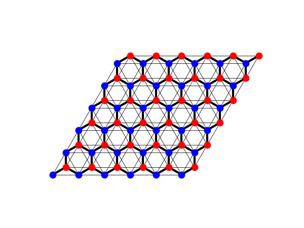
The Haldane model on a \(6\times6\)-cell flake, bond widths proportional to the amplitudes: the honeycomb lattice’s two sublattices (‘a’ and ‘b’, in two colours), the nearest-neighbour hopping (thick) and the second-neighbour hoppings \(\pm it_2\) (thin).

fig_lat = Plot(haldane_flake(6)).lattice(plt_hop=True, ms=10, figsize=(6, 4.5))

Clean flake: C in the bulk, -C on the edge

clean = haldane_flake(14)
marker = clean.get_local_chern_marker(0.)
print('Chern number {:.3f}; bulk marker {:.3f}; total {:.1e}.'
          .format(chern, marker[bulk(clean.lat)].mean(), marker.sum()))
assert abs(marker[bulk(clean.lat)].mean() - chern) < 0.02
assert abs(marker.sum()) < 1e-8

fig, ax = plt.subplots(figsize=(6, 5))
sc = ax.scatter(clean.lat.coor['x'], clean.lat.coor['y'], c=marker, cmap='RdBu', vmin=-2, vmax=2, s=20)
fig.colorbar(sc, ax=ax, label='local Chern marker')
ax.set_aspect('equal')
ax.axis('off')
ax.set_title('Haldane flake: the Chern number, site by site')

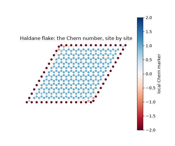
Chern number 1.000; bulk marker 1.000; total -4.3e-13.

Text(0.5, 1.0, 'Haldane flake: the Chern number, site by site')

Disorder: robust, until it closes the gap

strengths = [0., 1., 2., 8.]
means = []
for w in strengths:
    samples = [haldane_flake(12, w, seed) for seed in range(3)]
    means.append(np.mean([s.get_local_chern_marker(0.)[bulk(s.lat)].mean() for s in samples]))
print('Onsite disorder W:', strengths, '-> bulk marker:', np.round(means, 3))
assert abs(means[1] - chern) < 0.1          # weak disorder: still ~C
assert abs(means[-1]) < 0.3                  # strong disorder: trivial (localized)

Onsite disorder W: [0.0, 1.0, 2.0, 8.0] -> bulk marker: [1.    1.002 0.972 0.   ]