Magnetism of Triangular Graphene Nanoislands

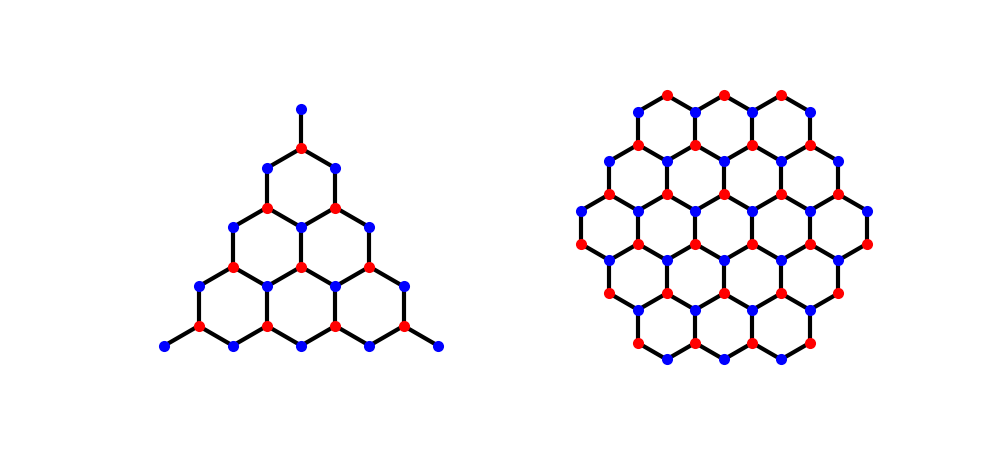
J. Fernández-Rossier and J. J. Palacios (2007) asked which graphene flakes are magnets, and found the answer in their shape. A triangle with zigzag edges has all three edges on the same sublattice, \(A\), and more \(A\) than \(B\) sites. A bipartite Hamiltonian then has (at least) \(N_Z = |A| - |B|\) states at exactly zero energy, all on sublattice \(A\) and concentrated on the edges. At half filling they hold \(N_Z\) electrons: like the open shell of an atom, they are filled with parallel spins (Hund’s rule), and the flake carries a spin \(S = N_Z/2\) – for any repulsion \(U\), however small, while a hexagonal flake needs \(U\) above a threshold. This is Lieb’s theorem made concrete: the moment grows with the size of the triangle. Triangular nanographenes (the “triangulenes”) were synthesized and seen to be magnetic in 2017-2021.

triangle_zigzag() cuts the flakes; hubbard_mean_field() solves the Hubbard model.

import numpy as np
import matplotlib.pyplot as plt

from tbkit.graphene import GrapheneLattice
from tbkit.meanfield import hubbard_mean_field
from tbkit.plot import Plot
from tbkit.system import System


def flake(shape, n):
    lat = GrapheneLattice()
    getattr(lat, shape)(n)
    sys = System(lat)
    sys.set_hopping([{'n': 1, 't': -1.}])
    sys.get_ham()
    return lat, sys


def ground_state(lat, sys, U, starts=2):
    '''Lowest-energy mean-field solution: a start polarized on sublattice
    A, and random ones.'''
    a = lat.coor['tag'] == 'a'
    up = np.where(a, 0.7, 0.3)
    results = [hubbard_mean_field(sys.ham, U, lat.sites, n_up=up, n_dn=1 - up, max_iter=100000)]
    results += [hubbard_mean_field(sys.ham, U, lat.sites, seed=seed, max_iter=100000) for seed in range(starts)]
    return min(results, key=lambda r: r.energy)

The two flakes

A zigzag triangle (left): all three edges end on sublattice A (tag ‘a’), so A has more sites than B. A zigzag hexagon (right) alternates A and B edges and keeps the two sublattices balanced.

fig_lat, axes_lat = plt.subplots(1, 2, figsize=(10, 4.5))
Plot(flake('triangle_zigzag', 5)[1]).lattice(plt_hop=True, ms=8, ax=axes_lat[0])
Plot(flake('hexagon_zigzag', 3)[1]).lattice(plt_hop=True, ms=8, ax=axes_lat[1])

<Figure size 1000x450 with 2 Axes>

Zero modes: one per extra A site

print('  n  sites  |A|-|B|  zero modes  S (U = 0.1|t|)  S (U = 2|t|)')
for n in (3, 5, 7, 9):
    lat, sys = flake('triangle_zigzag', n)
    a = lat.coor['tag'] == 'a'
    imbalance = int(a.sum() - (~a).sum())
    energies, states = np.linalg.eigh(sys.ham.toarray())
    zero = np.abs(energies) < 1e-8
    assert zero.sum() == imbalance and np.allclose(states[~a][:, zero], 0.)  # all on A
    spins = [abs(ground_state(lat, sys, U).total_spin) for U in (0.1, 2.)]
    assert np.allclose(spins, imbalance / 2, atol=1e-6)
    print('{:3d} {:6d} {:8d} {:11d} {:15.2f} {:13.2f}'.format(n, lat.sites, imbalance, zero.sum(), *spins))

n  sites  |A|-|B|  zero modes  S (U = 0.1|t|)  S (U = 2|t|)
3      9        3           3            1.50          1.50
5     25        5           5            2.50          2.50
7     49        7           7            3.50          3.50
9     81        9           9            4.50          4.50

A moment for any U: the zero modes, half filled

At small \(U\) the moment is the density of the zero modes, each filled by one spin-up electron: \(m_i \to \frac12\sum_z|\psi_z(i)|^2\). A zigzag hexagon of similar size has no zero mode and stays nonmagnetic at the same \(U\).

lat, sys = flake('triangle_zigzag', 9)
energies, states = np.linalg.eigh(sys.ham.toarray())
rho = np.sum(np.abs(states[:, np.abs(energies) < 1e-8]) ** 2, axis=1)
m_small = ground_state(lat, sys, 0.05).magnetization
deviation = np.max(np.abs(np.abs(m_small) - rho / 2))
print('Triangle, U = 0.05|t|: |m_i| = zero-mode density / 2 to {:.4f}.'.format(deviation))
assert deviation < 0.005
m_large = ground_state(lat, sys, 2.).magnetization

hexagon, sys_hex = flake('hexagon_zigzag', 4)
assert not np.any(np.abs(np.linalg.eigvalsh(sys_hex.ham.toarray())) < 1e-8)
m_hex = ground_state(hexagon, sys_hex, 0.1).magnetization
print('Hexagon ({} sites), U = 0.1|t|: largest |m_i| = {:.1e}.'.format(hexagon.sites, np.abs(m_hex).max()))
assert np.abs(m_hex).max() < 1e-6

fig, axes = plt.subplots(1, 3, figsize=(14, 4.5))
panels = ((rho / 2, 'zero-mode density / 2'),
              (m_small * np.sign(m_small.sum()), r'$m_i$, $U = 0.05|t|$'),
              (m_large * np.sign(m_large.sum()), r'$m_i$, $U = 2|t|$'))
for ax, (values, title) in zip(axes, panels):
    vmax = np.abs(values).max()
    sc = ax.scatter(lat.coor['x'], lat.coor['y'], c=values, cmap='RdBu_r', vmin=-vmax, vmax=vmax, s=40)
    fig.colorbar(sc, ax=ax, shrink=0.8)
    ax.set_aspect('equal')
    ax.axis('off')
    ax.set_title(title)
fig.suptitle('Triangular nanoisland, {} sites: S = {:.1f}'.format(lat.sites, abs(m_large.sum())))

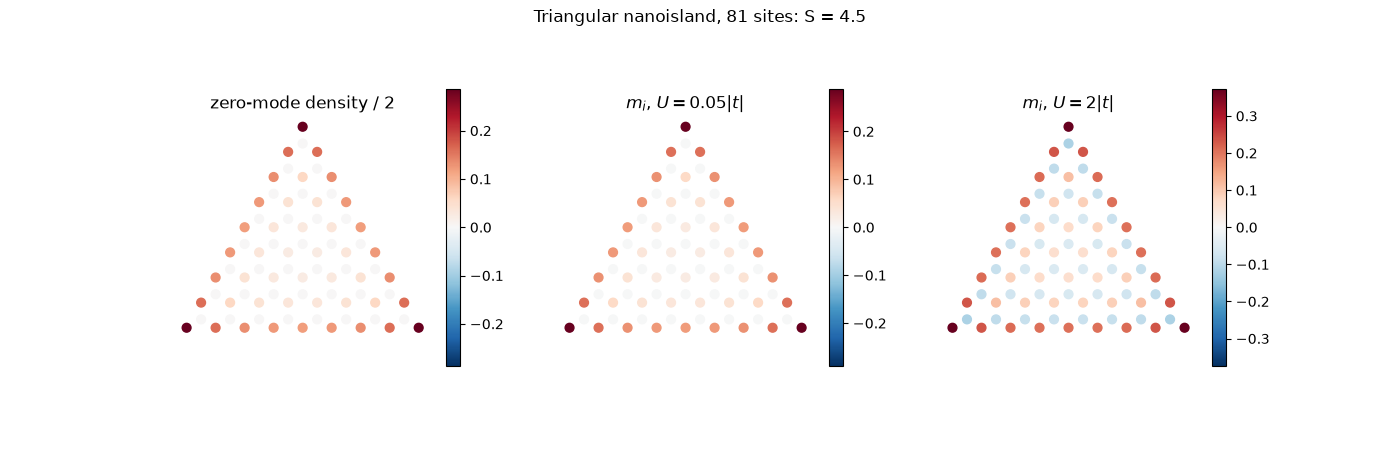
Triangle, U = 0.05|t|: |m_i| = zero-mode density / 2 to 0.0022.
Hexagon (96 sites), U = 0.1|t|: largest |m_i| = 5.7e-10.

Text(0.5, 0.98, 'Triangular nanoisland, 81 sites: S = 4.5')