The Modern Theory of Orbital Magnetization

The orbital magnetization of a crystal, \(\mathbf{M} = \frac{1}{2V}\int \mathbf{r}\times\mathbf{j}\), resisted a bulk formula for decades: the position operator is unbounded in a periodic solid, as for the polarization. In 2005 Thonhauser, Ceresoli, Vanderbilt and Resta (Wannier functions) and Xiao, Shi and Niu (semiclassical wavepackets) found it:

\[M = \frac{e}{h}\,\frac{1}{2\pi}\int_{BZ}d^2k\sum_nf_n\, \mathrm{Im}\langle\partial_xu_n|(H+E_n-2\mu)|\partial_yu_n\rangle\, .\]

Part of it is the self-rotation of the wavepackets; the rest, the term in \(\mu\), is carried by the edge currents, and in a Chern insulator it grows linearly as the Fermi level sweeps the gap – the edge states fill up. The slope is the Streda formula,

\[\frac{\partial M}{\partial\mu} = \frac{\partial n}{\partial B} = \sigma_{xy}\, ,\]

a Maxwell relation of the grand potential: the same number counts how many electrons a magnetic field pulls into the bulk.

orbital_magnetization() evaluates the formula on a k-mesh, for the Haldane model below, and a finite System in a magnetic field checks the Streda formula in real space.

import numpy as np
import matplotlib.pyplot as plt

import tbkit.lattices as lattices
from tbkit.bridges import finite_system
from tbkit.kspace import KSpace
from tbkit.plot import Plot


def haldane(M, t2=0.2):
    '''Haldane model: nearest-neighbour t = 1, i t2 on the second neighbours, mass +-M.'''
    hal = KSpace(lattices.honeycomb())
    hal.set_hopping([{'i': 0, 'j': 1, 'R': R, 't': 1.} for R in [(0, 0), (-1, 0), (0, -1)]])
    for R in [(0, 1), (-1, 0), (1, -1)]:
        hal.set_hopping([{'i': 0, 'j': 0, 'R': R, 't': 1j*t2}, {'i': 1, 'j': 1, 'R': R, 't': -1j*t2}])
    hal.set_onsite({'a': M, 'b': -M})
    return hal

The lattice

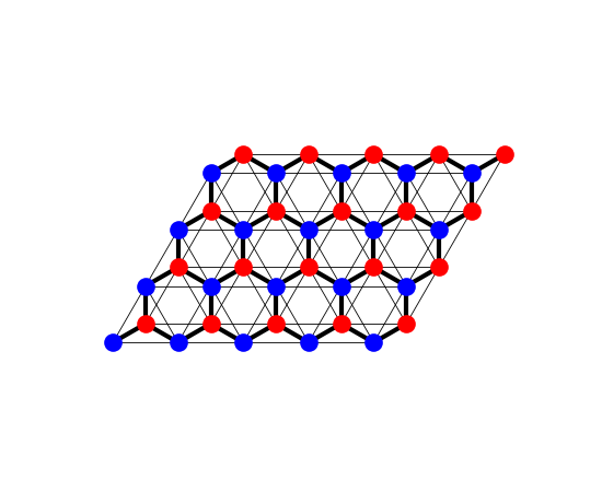
The Haldane model on a patch of \(5\times4\) cells (finite_system()), each bond drawn with a width proportional to its amplitude: the honeycomb lattice’s two sublattices (‘a’ and ‘b’, in two colours), the nearest-neighbour hopping \(t\) (thick) and the complex second-neighbour hoppings \(\pm it_2\) within each sublattice (thin), which break time-reversal symmetry.

fig_lat = Plot(finite_system(haldane(0.3), (5, 4))).lattice(plt_hop=True, ms=12, figsize=(5.5, 4.5))

Magnetization across the spectrum

In the topological phase (\(C = 1\)) the magnetization rises with slope exactly 1 (\(e/h\)) across the gap; in the trivial phase it is flat there. Empty and full bands carry none.

mu = np.linspace(-3.6, 3.6, 361)
phases = {'topological, M = 0.3': haldane(0.3), 'trivial, M = 1.5': haldane(1.5)}
mag = {name: hal.orbital_magnetization(mu, nk=120) for name, hal in phases.items()}

for name, hal in phases.items():
    en = hal.mesh_bands(120)
    in_gap = (mu > en[:, 0].max() + 0.02) & (mu < en[:, 1].min() - 0.02)
    slope = np.diff(mag[name][in_gap]) / np.diff(mu[in_gap])
    chern = hal.hall_conductivity(mu[in_gap][0], nk=120)
    print('{}: dM/dmu in the gap from {:.6f} to {:.6f}, sigma_xy = {:.6f}'.format(
        name, slope.min(), slope.max(), chern))
    assert np.allclose(slope, chern, atol=1e-6)
    assert mag[name][0] == 0. and abs(mag[name][-1]) < 1e-10

fig, ax = plt.subplots(figsize=(7, 4.5))
for (name, m), color in zip(mag.items(), ('C0', 'C3')):
    ax.plot(mu, m, color=color, label=name)
ax.axhline(0., color='k', lw=0.5)
ax.set_xlabel(r'$\mu$')
ax.set_ylabel(r'$M$ ($e/h$ $\times$ energy)')
ax.set_title('Haldane model: orbital magnetization')
ax.legend()

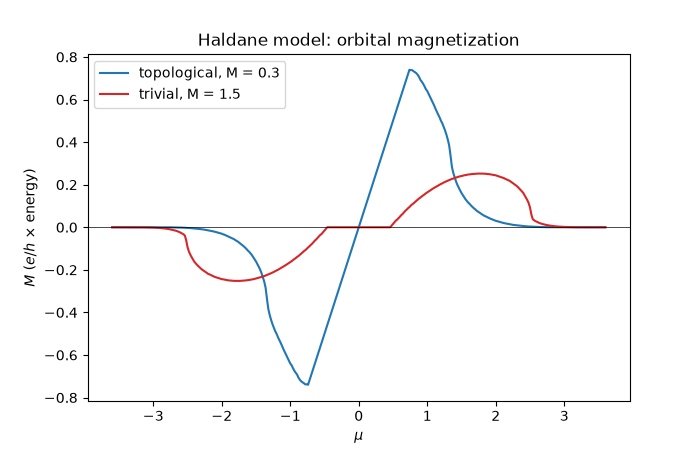
topological, M = 0.3: dM/dmu in the gap from 1.000000 to 1.000000, sigma_xy = 1.000000
trivial, M = 1.5: dM/dmu in the gap from -0.000000 to 0.000000, sigma_xy = 0.000000

<matplotlib.legend.Legend object at 0x10f07dfd0>

The Streda formula on a flake

A weak field \(B\) (flux density \(\alpha\) in flux quanta per unit area) at fixed \(\mu\) in the gap pulls electrons into the bulk of a Chern insulator: \(\Delta n = \sigma_{xy}\,\alpha\). Counting them in the middle of a 20 x 20 flake, away from its edge states, gives the slope of \(M(\mu)\) above to \(10^{-4}\).

hal = phases['topological, M = 0.3']
slope = (hal.orbital_magnetization(0.05, nk=120) - hal.orbital_magnetization(-0.05, nk=120)) / 0.1
alphas = np.array([-0.006, -0.003, 0., 0.003, 0.006])
counts = []
for alpha in alphas:
    sys = finite_system(hal, (20, 20))
    if alpha:
        sys.set_magnetic_field(alpha)
    sys.get_ham()
    sys.get_eig(eigenvec=True)
    x, y = sys.lat.coor['x'], sys.lat.coor['y']
    inside = np.hypot(x - x.mean(), y - y.mean()) < 6.
    counts.append(sys.get_charge_density(0.)[inside].sum())
area = inside.sum() / 2 * abs(np.linalg.det(np.array(hal.lat.prim_vec)))
density = (np.array(counts) - counts[2]) / area
dn_dalpha = np.polyfit(alphas, density, 1)[0]
print('dM/dmu (k-space) = {:.6f}, dn/dalpha (flake) = {:.6f}'.format(slope, dn_dalpha))
assert abs(dn_dalpha - slope) < 1e-4

fig2, ax2 = plt.subplots(figsize=(6, 4))
ax2.plot(alphas, density, 'o', label='flake, bulk region')
ax2.plot(alphas, slope * alphas, 'k--', lw=1, label=r'$\alpha\,\partial M/\partial\mu$ (k-space)')
ax2.set_xlabel(r'flux density $\alpha$ (flux quanta per unit area)')
ax2.set_ylabel(r'$\Delta n$ (electrons per unit area)')
ax2.set_title(r'Streda: $\partial n/\partial B = \partial M/\partial\mu$')
ax2.legend()

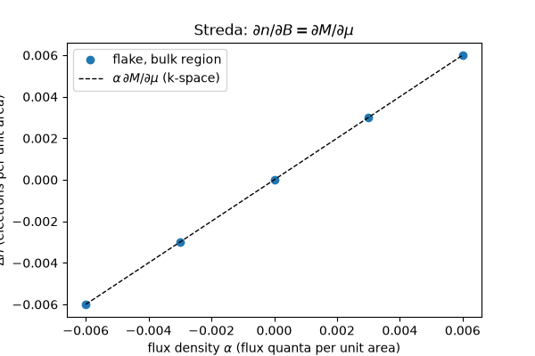
dM/dmu (k-space) = 1.000000, dn/dalpha (flake) = 0.999990

<matplotlib.legend.Legend object at 0x10f450d70>