Monkhorst-Pack k-Point Grids

Total energies, charge densities and every ground-state property of a crystal are averages over the Brillouin zone, \(\bar f = \frac{1}{V_{BZ}}\int f(\mathbf{k})\,d\mathbf{k}\). H. J. Monkhorst and J. D. Pack (1976) replaced the integral by the mean over a uniform grid of \(q\) points along each reciprocal vector, \(u_r = (2r - q - 1)/2q\), \(r = 1, \dots, q\). A smooth periodic function is a Fourier series \(f(\mathbf{k}) = \sum_\mathbf{R} f_\mathbf{R}e^{i\mathbf{k}\cdot\mathbf{R}}\), and such a grid averages every term to zero except those with all \(R_i\) multiples of \(q\): it integrates exactly every Fourier component of range below \(q\) lattice vectors. For an insulator the components decay exponentially, and so does the error. For even \(q\) the grid is shifted off \(\Gamma\), and its points fall into fewer orbits of the point group, so fewer have to be computed. Monkhorst-Pack grids have been the default k-point sampling of band-structure codes ever since.

tbkit.kspace.KSpace.mesh_grid() builds the \(\Gamma\)-centred grid (fractional coordinates \(r/q\)) or, with monkhorst_pack=True, the Monkhorst-Pack one. For odd \(q\) the two are the same points; for even \(q\) the Monkhorst-Pack grid is shifted by half a step.

import numpy as np
import matplotlib.pyplot as plt

import tbkit.lattices as lattices
from tbkit.bridges import finite_system
from tbkit.kspace import KSpace
from tbkit.plot import Plot
from tbkit.system import System


def grid(ks, q, monkhorst_pack):
    '''The k-points of a q x q grid: Gamma-centred, or Monkhorst-Pack.'''
    return ks.mesh_grid(int(q), monkhorst_pack=monkhorst_pack)[1]


t = 1.
square = KSpace(lattices.square())
square.set_hopping([{'n': 1, 't': -t}])

The lattices

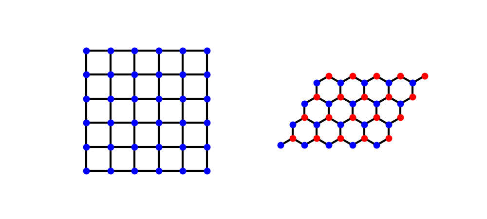
The square lattice (left, finite_system() of the model above), and the honeycomb lattice of gapped graphene (right, sublattices ‘a’ and ‘b’ in two colours), each with its nearest-neighbour bonds.

fig_lat, axes_lat = plt.subplots(1, 2, figsize=(10, 4.5))
Plot(finite_system(square, (6, 6))).lattice(plt_hop=True, ms=10, ax=axes_lat[0])
patch = lattices.honeycomb()
patch.get_lattice(n1=5, n2=4)
vis = System(patch)
vis.set_hopping([{'n': 1, 't': 1.}])
Plot(vis).lattice(plt_hop=True, ms=10, ax=axes_lat[1])

<Figure size 1000x450 with 2 Axes>

Exact moments of the band

On the square lattice, \(E^p(\mathbf{k})\) contains Fourier components up to range \(p\), and its average counts the closed walks of \(p\) steps: \(\overline{E^2} = 4t^2\), \(\overline{E^4} = 36t^4\). A \(q \times q\) grid gets \(\overline{E^p}\) exactly as soon as \(q > p\). Below that, the components with \(R_i = \pm q\) are aliased: they add \(+1\) per term on the \(\Gamma\)-centred grid, and \((-1)^{R_x/q + R_y/q}\) on the shifted one.

moments = {2: 4., 4: 36.}
for q in range(2, 7):
    row = []
    for mp in (False, True):
        en = square.get_bands(grid(square, q, mp))[:, 0]
        row.append([np.mean(en ** p) for p in moments])
    print('q = {}:  Gamma-centred <E^2>, <E^4> = {:5.1f} {:5.1f}   Monkhorst-Pack = {:5.1f} {:5.1f}'
          .format(q, *row[0], *row[1]))
    for mp in (0, 1):
        for value, (p, exact) in zip(row[mp], moments.items()):
            if q > p:
                assert np.isclose(value, exact * t ** p)
assert np.isclose(np.mean(square.get_bands(grid(square, 4, False))[:, 0] ** 4), 40.)   # +4 aliased
assert np.isclose(np.mean(square.get_bands(grid(square, 4, True))[:, 0] ** 4), 32.)    # -4 aliased

q = 2:  Gamma-centred <E^2>, <E^4> =   8.0 128.0   Monkhorst-Pack =   0.0   0.0
q = 3:  Gamma-centred <E^2>, <E^4> =   4.0  36.0   Monkhorst-Pack =   4.0  36.0
q = 4:  Gamma-centred <E^2>, <E^4> =   4.0  40.0   Monkhorst-Pack =   4.0  32.0
q = 5:  Gamma-centred <E^2>, <E^4> =   4.0  36.0   Monkhorst-Pack =   4.0  36.0
q = 6:  Gamma-centred <E^2>, <E^4> =   4.0  36.0   Monkhorst-Pack =   4.0  36.0

Insulators converge exponentially, metals do not

The band energy of the filled lower band of gapped graphene (staggered onsite \(\pm\Delta\), \(\Delta = t\)) is a smooth function of \(\mathbf{k}\), and the grid average converges exponentially: to \(10^{-14}\) on a \(24\times24\) grid. In a metal the occupation \(\theta(E_F - E(\mathbf{k}))\) jumps at the Fermi surface, its Fourier components decay only as a power, and so does the error: about \(q^{-2}\) for the half-filled square lattice, whose band energy is \(-8t/\pi^2\) per site. That slow convergence is why metals need dense grids, smearing, or the tetrahedron method.

gapped = KSpace(lattices.honeycomb())
gapped.set_hopping([{'n': 1, 't': -t}])
gapped.set_onsite({'a': t, 'b': -t})
e_insulator = np.mean(gapped.mesh_bands(96)[:, 0])
e_metal = -8. * t / np.pi ** 2

qs = np.array([4, 6, 8, 12, 16, 24, 32, 48, 64])
err_ins, err_met = [], []
for q in qs:
    err_ins.append(abs(np.mean(gapped.get_bands(grid(gapped, q, True))[:, 0]) - e_insulator))
    err_met.append(abs(np.mean(np.minimum(square.get_bands(grid(square, q, True))[:, 0], 0.)) - e_metal))
err_ins, err_met = np.array(err_ins), np.array(err_met)
for q, ei, em in zip(qs, err_ins, err_met):
    print('q = {:2d}: insulator error {:.1e}, metal error {:.1e}'.format(q, ei, em))
assert err_ins[qs == 24][0] < 1e-13
assert err_met[qs == 64][0] > 1e-4
slope = np.polyfit(np.log(qs[3:]), np.log(err_met[3:]), 1)[0]
print('metal: error ~ q^{:.2f}'.format(slope))
assert -2.3 < slope < -1.7

fig_conv, ax = plt.subplots(figsize=(6.5, 4.5))
ax.semilogy(qs, np.maximum(err_ins, 1e-16), 'o-', label='insulator (gapped graphene)')
ax.semilogy(qs, err_met, 's-', label='metal (half-filled square lattice)')
ax.semilogy(qs, err_met[-1] * (qs / qs[-1]) ** -2., 'k--', lw=1, label=r'$\propto q^{-2}$')
ax.set_xlabel(r'grid $q\times q$')
ax.set_ylabel('error of the band energy per cell')
ax.set_title('Brillouin-zone sampling error')
ax.legend()
fig_conv.tight_layout()

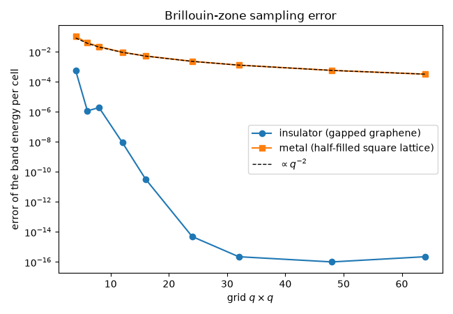
q =  4: insulator error 5.5e-04, metal error 1.0e-01
q =  6: insulator error 1.2e-06, metal error 4.1e-02
q =  8: insulator error 1.9e-06, metal error 2.2e-02
q = 12: insulator error 9.1e-09, metal error 9.5e-03
q = 16: insulator error 3.3e-11, metal error 5.3e-03
q = 24: insulator error 4.9e-15, metal error 2.3e-03
q = 32: insulator error 2.2e-16, metal error 1.3e-03
q = 48: insulator error 0.0e+00, metal error 5.8e-04
q = 64: insulator error 2.2e-16, metal error 3.3e-04
metal: error ~ q^-2.01

Fewer irreducible points

The square lattice has the 8 symmetries of \(C_{4v}\). A \(4\times4\) \(\Gamma\)-centred grid falls into 6 orbits, with \(\Gamma\), \(X\) and \(M\) among them. The Monkhorst-Pack grid avoids the high-symmetry points and falls into 3: the special points \((1,1)\), \((1,3)\) and \((3,3)\) in units of \(\pi/4a\), with weights 1/4, 1/2 and 1/4. It needs half the diagonalizations for the same Fourier accuracy.

def irreducible(kpts):
    '''Orbits under C4v: fold into the zone, then |kx|, |ky| sorted.'''
    frac = (kpts / (2 * np.pi) + 0.5) % 1. - 0.5
    rep = np.round(np.sort(np.abs(frac), axis=1), 9)
    return np.unique(rep, axis=0, return_counts=True)


for q in (4, 8):
    n_gamma = len(irreducible(grid(square, q, False))[0])
    n_mp = len(irreducible(grid(square, q, True))[0])
    print('{}x{} grid: {} irreducible points Gamma-centred, {} Monkhorst-Pack'.format(q, q, n_gamma, n_mp))
    assert n_mp < n_gamma
special, weights = irreducible(grid(square, 4, True))
assert np.allclose(special * 8, [[1, 1], [1, 3], [3, 3]])
assert np.allclose(weights / 16, [0.25, 0.5, 0.25])
# the three special points, with their weights, give <E^2> exactly
e_special = square.get_bands(special * 2 * np.pi)[:, 0]
assert np.isclose(np.sum(weights / 16 * e_special ** 2), 4. * t ** 2)

fig_grid, axes = plt.subplots(1, 2, figsize=(9, 4.5))
for ax, shifted, title in zip(axes, (False, True), (r'$\Gamma$-centred $4\times4$', r'Monkhorst-Pack $4\times4$')):
    kpts = (grid(square, 4, shifted) / (2 * np.pi) + 0.5) % 1. - 0.5
    for axis in (0, 1):      # draw the points on the zone boundary on both of its sides
        edge = np.isclose(kpts[:, axis], -0.5)
        kpts = np.vstack([kpts, kpts[edge] + np.eye(2)[axis]])
    reps, counts = irreducible(grid(square, 4, shifted))
    ax.add_patch(plt.Polygon([[0, 0], [0.5, 0], [0.5, 0.5]], color='#dce8f5'))
    ax.plot(kpts[:, 0], kpts[:, 1], 'o', color='#3b76af', ms=7)
    ax.plot(reps[:, 1], reps[:, 0], 'o', color='#c53a32', ms=11, mfc='none', mew=2)
    ax.set_xlim(-0.55, 0.55)
    ax.set_ylim(-0.55, 0.55)
    ax.set_aspect('equal')
    ax.set_xlabel(r'$k_x a/2\pi$')
    ax.set_ylabel(r'$k_y a/2\pi$')
    ax.set_title('{}: {} irreducible'.format(title, len(reps)))
fig_grid.tight_layout()

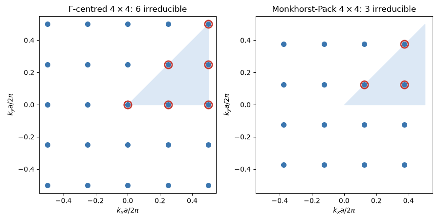
4x4 grid: 6 irreducible points Gamma-centred, 3 Monkhorst-Pack
8x8 grid: 15 irreducible points Gamma-centred, 10 Monkhorst-Pack