Zigzag Edge States of Graphene Ribbons

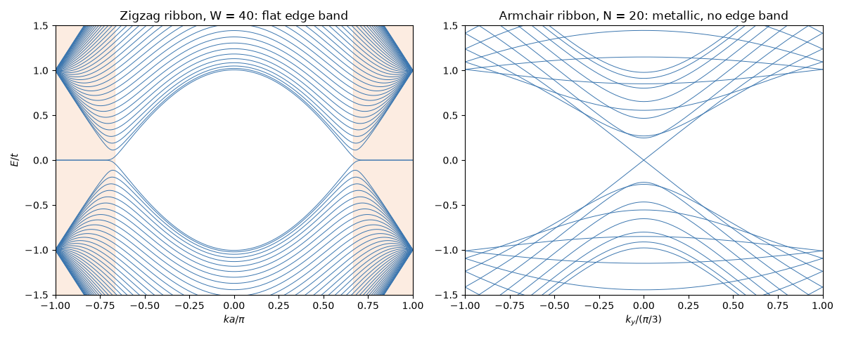
M. Fujita, K. Wakabayashi, K. Nakada and K. Kusakabe (1996) cut graphene into ribbons and found that the shape of the edge decides the low-energy physics. A ribbon with zigzag edges has a band of states at exactly \(E = 0\), localized at the edges, over a third of its Brillouin zone, \(2\pi/3 \le |ka| \le \pi\). Each such state lives on one sublattice only, with amplitude \((-2\cos\tfrac{ka}{2})^n\) on the \(n\)-th zigzag chain from its edge: localized when \(|2\cos\tfrac{ka}{2}| < 1\), most strongly at the zone boundary. The flat band piles up states at the Fermi level, a peak in the density of states that makes the edges magnetic once electrons interact. A ribbon with armchair edges has no edge states. Nakada et al. showed that it is metallic only when its number \(N\) of dimer lines is \(N = 3m + 2\), and gapped otherwise.

tbkit.kspace.ribbon() cuts the ribbon out of any 2D KSpace model: periodic along one primitive vector, \(W\) cells wide along the other.

import numpy as np
import matplotlib.pyplot as plt

import tbkit.lattices as lattices
from tbkit.lattice import Lattice
from tbkit.kspace import ribbon
from tbkit.neighbours import neighbour_hoppings
from tbkit.system import System
from tbkit.plot import Plot


t = 1.
lat = lattices.honeycomb()          # nearest-neighbour distance 1, a = sqrt(3)
a = np.linalg.norm(lat.prim_vec[0])
hop = neighbour_hoppings(lat, [{'n': 1, 't': -t}], False)

The zigzag ribbon

Periodic along \(\mathbf{a}_1\), the zigzag direction, and finite across. Drawn 6 cells wide:

rib_small = ribbon(lat, hop, width=6, direction=1)
# ribbon() stacks its rows along a2, which has a component along a1 too:
# sliding each site back by whole multiples of a1 draws the same lattice as
# a straight strip, periodic left-to-right with zigzag edges top and bottom.
a1 = np.array(rib_small.lat.prim_vec[0])
folded = [{'tag': d['tag'],
           'r0': tuple(np.array(d['r0']) - round(np.dot(d['r0'], a1) / (a1 @ a1)) * a1)}
          for d in rib_small.lat.unit_cell]
lat_draw = Lattice(unit_cell=folded, prim_vec=rib_small.lat.prim_vec)
lat_draw.get_lattice(n1=9)
vis = System(lat_draw)
vis.set_hopping([{'n': 1, 't': -t}])
fig_rib = Plot(vis).lattice(plt_hop=True, ms=9, figsize=(8, 4.5))

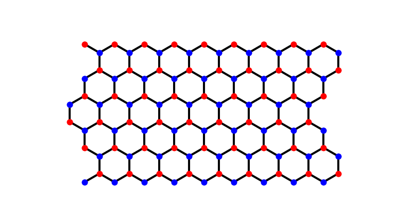
The ribbon diagonalized is 40 cells wide. Its bands are those of graphene projected on \(k_x\), plus one band at \(E = 0\) that joins the projections of the two Dirac points \(ka = \pm2\pi/3\) through the zone boundary. On that band the two edge states (one per edge) split only by an amount exponentially small in the width.

width = 40
zigzag = ribbon(lat, hop, width=width, direction=1)
ka = np.linspace(-np.pi, np.pi, 601)
en, vec = zigzag.get_bands(ka[:, None] / a, eigenvec=True)
lowest = np.sort(np.abs(en), axis=1)[:, :2]
deep = np.abs(ka) >= 0.75 * np.pi
print('|E| of the two edge states for |ka| >= 0.75 pi: at most {:.1e}'.format(lowest[deep].max()))
assert lowest[deep].max() < 1e-4
outside = np.abs(ka) <= 0.6 * np.pi
print('lowest |E| for |ka| <= 0.6 pi: at least {:.3f}'.format(lowest[outside, 0].min()))
assert lowest[outside, 0].min() > 0.03

|E| of the two edge states for |ka| >= 0.75 pi: at most 9.4e-06
lowest |E| for |ka| <= 0.6 pi: at least 0.190

Decay into the ribbon

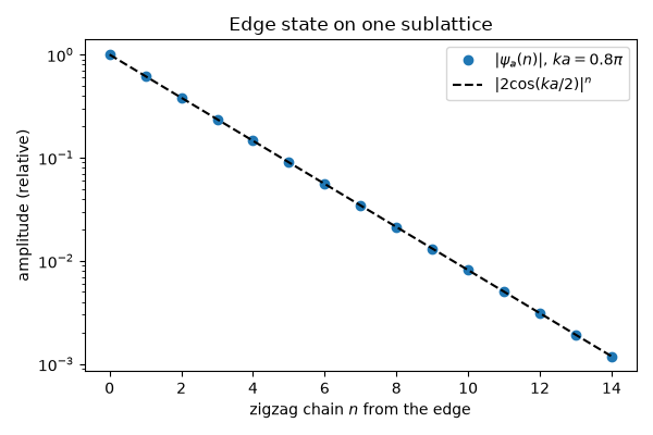
At \(ka = 0.8\pi\), the zero-energy state sits on the a sites of one edge, with nothing on the b sites, and its amplitude falls by \(|2\cos(0.4\pi)| = 0.618\) from one zigzag chain to the next.

i_k = np.argmin(np.abs(ka - 0.8 * np.pi))
psi = np.abs(vec[i_k][:, np.argmin(np.abs(en[i_k]))].reshape(width, 2))   # rows x (a, b)
# the zero-energy pair mixes the two edges: the a sites carry the state of
# the edge at row 0, the b sites that of the opposite edge
edge = psi[:, 0]
assert edge[0] > edge[-1] and np.all(psi[:5, 1] < 1e-6 * edge[0])
ratio = edge[1:8] / edge[:7]
print('decay ratio per zigzag chain: {}, expected {:.4f}'.format(
    np.array2string(ratio, precision=4), abs(2 * np.cos(0.4 * np.pi))))
assert np.allclose(ratio, abs(2 * np.cos(0.4 * np.pi)), rtol=1e-3)

decay ratio per zigzag chain: [0.618 0.618 0.618 0.618 0.618 0.618 0.618], expected 0.6180

A third of the states at \(E = 0\)

The flat band carries \(1/3\) of a state per edge and per unit length \(a\). Its contribution to the density of states is a peak at \(E = 0\) that does not shrink as the ribbon gets wider, while bulk graphene has \(\rho(0) = 0\).

ka_fine = np.linspace(-np.pi, np.pi, 3001)[:-1]
en_fine = zigzag.get_bands(ka_fine[:, None] / a)
fraction = np.mean(np.sum(np.abs(en_fine) < 1e-2, axis=1) / 2.)
print('edge states per edge and per k: {:.3f} (expected 1/3, minus the finite-width tail)'.format(fraction))
assert abs(fraction - 1 / 3) < 0.03

edge states per edge and per k: 0.312 (expected 1/3, minus the finite-width tail)

Armchair ribbons: no edge states, and the 3m + 2 rule

A rectangular cell of four sites, periodic along \(y\), cut \(W\) cells wide along \(x\), gives armchair edges with \(N = 2W\) dimer lines. There is no flat band, and the ribbon is metallic (gap at \(k = 0\) closed) exactly when \(N = 3m + 2\).

s3 = np.sqrt(3.)
rect = Lattice(unit_cell=[{'tag': 'a', 'r0': (0., 0.)}, {'tag': 'b', 'r0': (s3 / 2, 0.5)},
                          {'tag': 'a', 'r0': (s3 / 2, 1.5)}, {'tag': 'b', 'r0': (0., 2.)}],
               prim_vec=[(s3, 0.), (0., 3.)])
rect_hop = neighbour_hoppings(rect, [{'n': 1, 't': -t}], False)
widths = np.arange(3, 12)
gaps = []
for w in widths:
    arm = ribbon(rect, rect_hop, width=int(w), direction=0)
    gaps.append(2 * np.abs(arm.get_bands(np.linspace(-np.pi / 3, np.pi / 3, 121)[:, None])).min())
gaps = np.array(gaps)
dimer_lines = 2 * widths
for n, g in zip(dimer_lines, gaps):
    print('armchair N = {:2d} (N mod 3 = {}): gap {:.4f}'.format(n, n % 3, g))
metallic = dimer_lines % 3 == 2
assert np.all(gaps[metallic] < 1e-10)
assert np.all(gaps[~metallic] > 0.1)

armchair = ribbon(rect, rect_hop, width=10, direction=0)
ky = np.linspace(-np.pi / 3, np.pi / 3, 301)
en_arm = armchair.get_bands(ky[:, None])

fig, (ax1, ax2) = plt.subplots(1, 2, figsize=(12, 4.8))
ax1.plot(ka / np.pi, en, color='#3b76af', lw=0.7)
ax1.axvspan(2 / 3, 1, color='#ef8636', alpha=0.15)
ax1.axvspan(-1, -2 / 3, color='#ef8636', alpha=0.15)
ax1.set_xlim(-1, 1)
ax1.set_ylim(-1.5, 1.5)
ax1.set_xlabel(r'$ka/\pi$')
ax1.set_ylabel('$E/t$')
ax1.set_title('Zigzag ribbon, W = {}: flat edge band'.format(width))
ax2.plot(ky * 3 / np.pi, en_arm, color='#3b76af', lw=0.7)
ax2.set_xlim(-1, 1)
ax2.set_ylim(-1.5, 1.5)
ax2.set_xlabel(r'$k_y/(\pi/3)$')
ax2.set_title('Armchair ribbon, N = 20: metallic, no edge band')
fig.tight_layout()

fig_decay, ax = plt.subplots(figsize=(6, 4))
rows = np.arange(15)
ax.semilogy(rows, edge[:15] / edge[0], 'o', label=r'$|\psi_a(n)|$, $ka = 0.8\pi$')
ax.semilogy(rows, abs(2 * np.cos(0.4 * np.pi)) ** rows, 'k--', label=r'$|2\cos(ka/2)|^n$')
ax.set_xlabel('zigzag chain $n$ from the edge')
ax.set_ylabel('amplitude (relative)')
ax.set_title('Edge state on one sublattice')
ax.legend()
fig_decay.tight_layout()

• 
• 

armchair N =  6 (N mod 3 = 0): gap 0.4940
armchair N =  8 (N mod 3 = 2): gap 0.0000
armchair N = 10 (N mod 3 = 1): gap 0.3383
armchair N = 12 (N mod 3 = 0): gap 0.2723
armchair N = 14 (N mod 3 = 2): gap 0.0000
armchair N = 16 (N mod 3 = 1): gap 0.2170
armchair N = 18 (N mod 3 = 0): gap 0.1878
armchair N = 20 (N mod 3 = 2): gap 0.0000
armchair N = 22 (N mod 3 = 1): gap 0.1597