Lieb’s Theorem: The Ferrimagnet of the Lieb Lattice

E. Lieb proved in 1989 one of the few exact results on the Hubbard model: on a bipartite lattice at half filling, for any repulsion \(U > 0\), the ground state has total spin

\[S = \frac{\bigl||A| - |B|\bigr|}{2}\, ,\]

set by the imbalance between the two sublattices alone. His own example is the lattice now named after him: a square lattice (sites \(A\)) with an extra site on every bond (sites \(B\)), so \(|B| = 2|A|\). Its middle band is exactly flat, at zero energy, and lives on \(B\) only; at half filling it is half filled, and the ground state is a ferrimagnet: moments up on \(B\), smaller ones down on \(A\), and a net spin of one half per unit cell.

The unrestricted mean-field solution (hubbard_mean_field()) is not exact, but its lowest-energy state obeys Lieb’s count. (Other self-consistent solutions exist, of lower spin and higher energy: random starts often find those, so several starts are compared.)

import numpy as np
import matplotlib.pyplot as plt

import tbkit.lattices as lattices
from tbkit.meanfield import hubbard_mean_field
from tbkit.plot import Plot
from tbkit.system import System


def lieb(n, periodic):
    lat = lattices.lieb()
    lat.get_lattice(n1=n, n2=n)
    sys = System(lat, periodic=periodic)
    sys.set_hopping([{'n': 1, 't': -1.}])
    sys.get_ham()
    return lat, sys


def ground_state(lat, sys, U, starts=2):
    '''Lowest-energy mean-field solution over several starts: random ones,
    and a staggered magnetization (up on B, down on A).'''
    a = lat.coor['tag'] == 'a'
    up = np.where(a, 0.3, 0.7)
    results = [hubbard_mean_field(sys.ham, U, lat.sites, n_up=up, n_dn=1 - up)]
    results += [hubbard_mean_field(sys.ham, U, lat.sites, seed=seed) for seed in range(starts)]
    return min(results, key=lambda r: r.energy)

The Lieb lattice

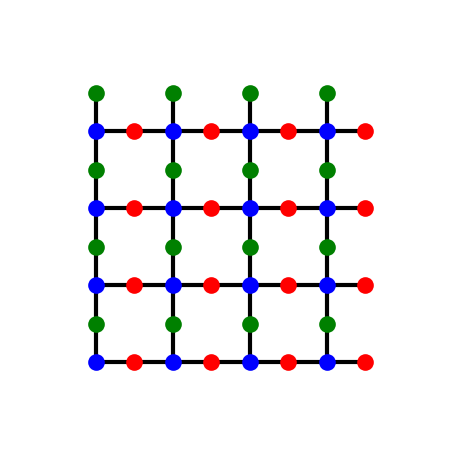
A square lattice with an extra site on every bond: per unit cell, one corner site (sublattice A, tag ‘a’) and two edge-centre sites (B, tags ‘b’ and ‘c’), so B has twice as many sites as A.

fig_lat = Plot(lieb(4, periodic=False)[1]).lattice(plt_hop=True, ms=12, figsize=(4.5, 4.5))

The flat band lives on B

# On a 5x5 torus (odd, so the k-mesh misses the point M where all three
# bands meet), the flat band holds one state per cell.
lat, sys = lieb(5, periodic=True)
a = lat.coor['tag'] == 'a'
energies, states = np.linalg.eigh(sys.ham.toarray())
flat = np.abs(energies) < 1e-8
assert flat.sum() == a.sum() and np.allclose(states[a][:, flat], 0.)
print('5x5 torus: {} sites, {} zero-energy states, all on B.'.format(lat.sites, flat.sum()))

5x5 torus: 75 sites, 25 zero-energy states, all on B.

Lieb’s count holds for every size and U

rows = []
for n, periodic in ((4, True), (5, True), (4, False), (5, False)):
    lat, sys = lieb(n, periodic)
    a = lat.coor['tag'] == 'a'
    lieb_spin = abs(lat.sites - 2 * a.sum()) / 2
    for U in (0.5, 2.):
        m = ground_state(lat, sys, U).magnetization
        assert np.isclose(abs(m.sum()), lieb_spin, atol=1e-6)
        # ferrimagnet: B and A moments opposite
        assert np.all(m[~a] * np.sign(m.sum()) > 0) and np.all(m[a] * np.sign(m.sum()) < 0)
        rows.append((n, 'torus' if periodic else 'open', lat.sites, a.sum(), (~a).sum(), U, abs(m.sum())))
print('  n  edges  sites  |A|  |B|    U    S')
for row in rows:
    print('{:3d} {:>6} {:6d} {:4d} {:4d} {:4.1f} {:5.1f}'.format(*row))

n  edges  sites  |A|  |B|    U    S
4  torus     48   16   32  0.5   8.0
4  torus     48   16   32  2.0   8.0
5  torus     75   25   50  0.5  12.5
5  torus     75   25   50  2.0  12.5
4   open     48   16   32  0.5   8.0
4   open     48   16   32  2.0   8.0
5   open     75   25   50  0.5  12.5
5   open     75   25   50  2.0  12.5

The ferrimagnetic order

lat, sys = lieb(5, periodic=False)
m = ground_state(lat, sys, 2.).magnetization
fig, ax = plt.subplots(figsize=(5.5, 5))
vmax = np.abs(m).max()
sc = ax.scatter(lat.coor['x'], lat.coor['y'], c=m * np.sign(m.sum()), cmap='RdBu_r',
                        vmin=-vmax, vmax=vmax, s=80)
fig.colorbar(sc, ax=ax, label='$m_i$')
ax.set_aspect('equal')
ax.axis('off')
ax.set_title('Lieb lattice, {} sites, $U = 2|t|$: $S = {:.1f}$'.format(lat.sites, abs(m.sum())))

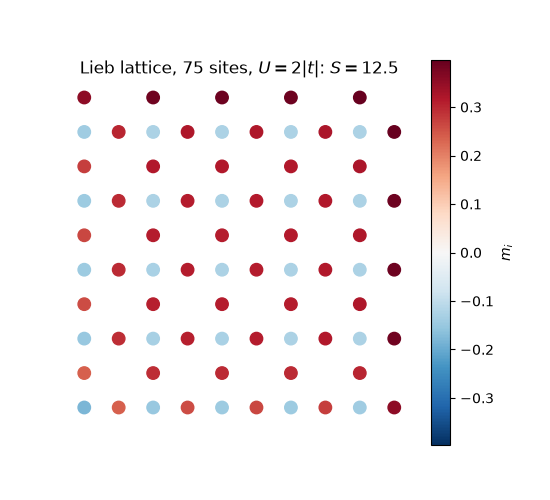
Text(0.5, 1.0, 'Lieb lattice, 75 sites, $U = 2|t|$: $S = 12.5$')