The Surface Green’s Function by Lopez Sancho Decimation#

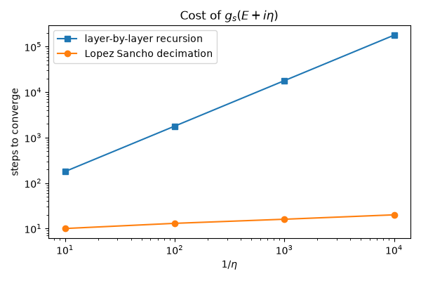
A surface is a crystal cut in half: periodic along the surface, but semi-infinite in depth. Its local density of states is $-\frac{1}{\pi}\mathrm{Im}\,G_{00}(E + i\eta)$, the Green’s function of the outermost layer, which depends on every layer below it. A finite slab only approximates it, with discrete levels and a second surface. The recursion $g = [E - h_0 - v\,g\,v^\dagger]^{-1}$, which adds one layer at a time, converges only as fast as the broadening $\eta$ damps the waves coming back from the bulk: $\sim1/\eta$ steps.

M. P. Lopez Sancho, J. M. Lopez Sancho and J. Rubio (1984, 1985) decimated instead. Each step eliminates every other layer, which leaves a chain of the same form with renormalized couplings, so step $n$ accounts for $2^n$ layers and the renormalized couplings vanish after a few tens of steps. This made surface Green’s functions a routine calculation: the surface states and resonances of photoemission, and the self-energies of the semi-infinite leads of quantum transport.

tbkit.transport.surface_green() decimates any chain of cells $(h_0, v)$, and tbkit.kspace.KSpace.surface_spectral_function() applies it to the surface of a periodic model.

import numpy as np
import matplotlib.pyplot as plt

from tbkit.lattice import Lattice
from tbkit.bridges import finite_system
from tbkit.kspace import KSpace
from tbkit.plot import Plot
from tbkit.system import System
from tbkit.transport import surface_green

The lattice#

The first crystal is a chain, one site per cell and a hopping $t$ between neighbours, cut at its left end and continuing forever to the right (ten sites drawn).

lat_vis = Lattice(unit_cell=[{'tag': 'a', 'r0': (0., 0.)}], prim_vec=[(1., 0.)])
lat_vis.get_lattice(n1=10)
vis = System(lat_vis)
vis.set_hopping([{'n': 1, 't': 1.}])
fig_lat = Plot(vis).lattice(plt_hop=True, ms=12, figsize=(7, 1.2))

The semi-infinite chain#

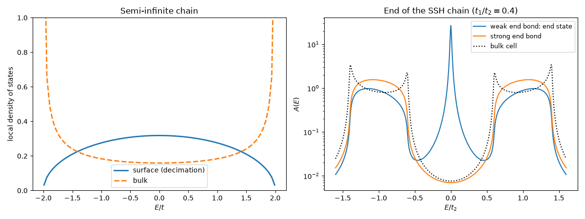
For a chain with hopping $t$ the recursion $g = 1/(E - t^2g)$ is a quadratic equation, and its retarded root is $g(E) = (E - i\sqrt{4t^2 - E^2})/2t^2$ inside the band. The surface density of states $\sqrt{4t^2 - E^2}/2\pi t^2$ vanishes at the band edges like a square root, where the bulk one, $1/\pi\sqrt{4t^2 - E^2}$, diverges.

t = 1.
energies = np.linspace(-1.99, 1.99, 81)
g_dec = np.array([surface_green([[0.]], [[t]], e)[0, 0] for e in energies])
g_exact = (energies - 1j * np.sqrt(4 * t ** 2 - energies ** 2)) / (2 * t ** 2)
print('Decimation vs closed form: max |g - g_exact| = {:.1e}'.format(np.abs(g_dec - g_exact).max()))
assert np.allclose(g_dec, g_exact, atol=1e-6)
rho_surface = -g_dec.imag / np.pi
assert np.allclose(rho_surface, np.sqrt(4 * t ** 2 - energies ** 2) / (2 * np.pi * t ** 2), atol=1e-6)

Decimation vs closed form: max |g - g_exact| = 5.0e-09

Twenty steps instead of $1/\eta$#

The number of decimation steps needed grows like $\log_2(1/\eta)$; the layer-by-layer recursion needs about $1/\eta$ iterations to reach the same Green’s function.

def decimation_steps(energy, eta):
    '''Fewest decimation steps for which surface_green converges.'''
    n = 1
    while True:
        try:
            return n, surface_green([[0.]], [[t]], energy, eta=eta, max_iter=n)[0, 0]
        except RuntimeError:
            n += 1


def recursion_steps(energy, eta, target, tol=1e-8):
    '''Iterations of g = 1/(E + i eta - t^2 g) from g = 0 until within tol of target.'''
    g, n = 0., 0
    while abs(g - target) > tol * abs(target):
        g = 1. / (energy + 1j * eta - t ** 2 * g)
        n += 1
    return n


etas = np.array([1e-1, 1e-2, 1e-3, 1e-4])
n_dec, n_rec = [], []
for eta in etas:
    steps, g = decimation_steps(0.7, eta)
    n_dec.append(steps)
    n_rec.append(recursion_steps(0.7, eta, g))
    print('eta = {:.0e}: {:3d} decimation steps, {:6d} recursion steps'.format(eta, n_dec[-1], n_rec[-1]))
n_dec, n_rec = np.array(n_dec), np.array(n_rec)
assert np.all(n_dec <= 25)
assert np.all(np.diff(n_dec) <= 4)                  # about log2(10) = 3.3 more per decade
assert n_rec[-1] > 100 * n_dec[-1]
assert np.allclose(n_rec[1:] / n_rec[:-1], 10., rtol=0.05)   # proportional to 1/eta

eta = 1e-01:  10 decimation steps,    179 recursion steps
eta = 1e-02:  13 decimation steps,   1784 recursion steps
eta = 1e-03:  16 decimation steps,  17844 recursion steps
eta = 1e-04:  20 decimation steps, 178437 recursion steps

A surface state: the end of an SSH chain#

The Su-Schrieffer-Heeger chain alternates hoppings $t_1$ (inside the cell) and $t_2$. When the chain ends on a weak bond ($|t_1| < |t_2|$), a state at $E = 0$ is bound to the end, with amplitude $(-t_1/t_2)^n$ on the $a$ site of cell $n$: a weight $1 - (t_1/t_2)^2$ on the outermost cell. It is a delta function in the surface spectral function, $A(0) = [1 - (t_1/t_2)^2]/\pi\eta$ at small $\eta$, with no bulk state at that energy. When the chain ends on a strong bond there is none. Here the crystal is the semi-infinite chain of cells $0, 1, 2, \dots$; side=-1 gives the opposite end.

def ssh(t1, t2):
    lat = Lattice(unit_cell=[{'tag': 'a', 'r0': (0., 0.)}, {'tag': 'b', 'r0': (0.5, 0.)}],
                  prim_vec=[(1., 0.)])
    ks = KSpace(lat)
    ks.set_hopping([{'i': 0, 'j': 1, 'R': (0,), 't': t1}, {'i': 1, 'j': 0, 'R': (1,), 't': t2}])
    return ks


eta = 1e-4
t1, t2 = 0.4, 1.

# Its first eight cells (:func:`~tbkit.bridges.finite_system`), orbitals
# a and b in two colours, bond widths proportional to the hoppings: the
# chain ends on the weak bond :math:`t_1`.
fig_ssh = Plot(finite_system(ssh(t1, t2), 8)).lattice(plt_hop=True, ms=7, c=4., figsize=(7, 1.2))

The end state’s weight, at both ends:

for side in (1, -1):
    weight = ssh(t1, t2).surface_spectral_function([[0.]], [0.], direction=0, side=side, eta=eta)[0, 0] * np.pi * eta
    print('t1/t2 = {}: end-state weight on the outer cell {:.4f} (side {:+d}), expected {:.4f}'.format(
        t1 / t2, weight, side, 1 - (t1 / t2) ** 2))
    assert np.isclose(weight, 1 - (t1 / t2) ** 2, rtol=1e-4)
trivial = ssh(t2, t1).surface_spectral_function([[0.]], [0.], direction=0, eta=eta)[0, 0] * np.pi * eta
print('t1/t2 = {}: weight at E = 0 {:.1e}'.format(t2 / t1, trivial))
assert trivial < 1e-6

e_grid = np.linspace(-1.6, 1.6, 641)
fig, (ax1, ax2) = plt.subplots(1, 2, figsize=(12, 4.5))
ax1.plot(energies, rho_surface, lw=2, label='surface (decimation)')
ax1.plot(energies, 1 / (np.pi * np.sqrt(4 * t ** 2 - energies ** 2)), '--', lw=2, label='bulk')
ax1.set_xlabel('$E/t$')
ax1.set_ylabel('local density of states')
ax1.set_ylim(0, 1.)
ax1.set_title('Semi-infinite chain')
ax1.legend()
for (a, b), label in (((t1, t2), 'weak end bond: end state'), ((t2, t1), 'strong end bond')):
    spec = ssh(a, b).surface_spectral_function([[0.]], e_grid, direction=0, eta=1e-2)[0]
    ax2.semilogy(e_grid, spec, lw=1.5, label=label)
ax2.semilogy(e_grid, ssh(t1, t2).surface_spectral_function([[0.]], e_grid, direction=0, eta=1e-2,
                                                           bulk=True)[0], 'k:', lw=1.5, label='bulk cell')
ax2.set_xlabel('$E/t_2$')
ax2.set_ylabel(r'$A(E)$')
ax2.set_title('End of the SSH chain ($t_1/t_2 = 0.4$)')
ax2.legend(fontsize=9)
fig.tight_layout()

fig_steps, ax = plt.subplots(figsize=(6, 4))
ax.loglog(1 / etas, n_rec, 's-', label='layer-by-layer recursion')
ax.loglog(1 / etas, n_dec, 'o-', label='Lopez Sancho decimation')
ax.set_xlabel(r'$1/\eta$')
ax.set_ylabel('steps to converge')
ax.legend()
ax.set_title(r'Cost of $g_s(E + i\eta)$')
fig_steps.tight_layout()

$Cost of $g_s(E + i\eta)$$

t1/t2 = 0.4: end-state weight on the outer cell 0.8400 (side +1), expected 0.8400
t1/t2 = 0.4: end-state weight on the outer cell 0.8400 (side -1), expected 0.8400
t1/t2 = 2.5: weight at E = 0 2.2e-08

Total running time of the script: (0 minutes 0.298 seconds)

Gallery generated by Sphinx-Gallery

The Surface Green’s Function by Lopez Sancho Decimation#

The lattice#

The semi-infinite chain#

Twenty steps instead of \(1/\eta\)#

A surface state: the end of an SSH chain#