Dynamic Localization and Coherent Destruction of Tunnelling

Dunlap and Kenkre (1986) found that an AC field \(F\cos\omega t\) on a chain does not simply shake its electrons: averaged over a period, it renormalizes the hopping,

\[t \to t\,J_0(F/\omega)\, ,\]

with \(J_0\) the Bessel function (lattice constant 1, \(\hbar = 1\)). At the zeros of \(J_0\), the first at \(F/\omega = 2.405\), the band collapses and a wavepacket no longer spreads: dynamic localization. Grossmann, Dittrich, Jung and Hänggi (1991) found the same suppression in a driven double well, \(H(t) = -t\sigma_x + \frac{A}{2}\cos(\omega t)\sigma_z\): at high frequency the two quasienergies are split by \(2t|J_0(A/\omega)|\), so the tunnelling stops at the zeros of \(J_0\) – coherent destruction of tunnelling. Both were observed with cold atoms in driven optical lattices (Lignier et al., 2007) and with light in curved waveguide arrays (Longhi et al., 2006; Della Valle et al., 2007).

On the chain, the field enters as the vector potential \(-(F/\omega)\sin\omega t\), \(H(k, t) = 2t\cos(k - (F/\omega)\sin\omega t)\). Its values at different times commute, so the Floquet band is exactly the time average \(2tJ_0(F/\omega)\cos k\), which DrivenKSpace recovers. For the double well, effective_hamiltonian() and quasienergies() give the renormalized tunnelling.

import numpy as np
import matplotlib.pyplot as plt
from scipy.special import j0, jn_zeros

import tbkit.lattices as lattices
from tbkit.bridges import finite_system
from tbkit.kspace import KSpace
from tbkit.plot import Plot
from tbkit.floquet import DrivenKSpace, effective_hamiltonian, evolution_operator, quasienergies

t = 1.
first_zero = jn_zeros(0, 1)[0]

Dynamic localization: the Floquet band of a chain in an AC field

chain = KSpace(lattices.chain())
chain.set_hopping([{'i': 0, 'j': 0, 'R': (1,), 't': t}])

# The chain: one site per unit cell and a nearest-neighbour hopping t.
fig_lat = Plot(finite_system(chain, 10)).lattice(plt_hop=True, ms=12, figsize=(7, 1.2))

An AC field \(F\cos\omega t\) shakes the chain; its quasienergy band is that of the static chain, with \(t\) renormalized by \(J_0(F/\omega)\).

omega = 5.
ks = np.linspace(-np.pi, np.pi, 61)


def floquet_band(ratio):
    '''The quasienergy band of the chain driven at F / omega = ratio.'''
    driven = DrivenKSpace(chain, lambda k, tt: np.array([[2 * t * np.cos(k[0] - ratio * np.sin(omega * tt))]]),
                                  2 * np.pi / omega, n_steps=64)
    return np.array([driven.get_ham([k])[0, 0].real for k in ks])


ratios = [0., 1., first_zero, 3.5]
bands = [floquet_band(r) for r in ratios]
for r, band in zip(ratios, bands):
    assert np.allclose(band, 2 * t * j0(r) * np.cos(ks), atol=1e-10)
widths = [np.ptp(band) for band in bands]
print('Floquet bandwidths:', np.round(widths, 6), ' 4t|J0(F/omega)|:', np.round(4 * t * np.abs(j0(ratios)), 6))
assert widths[2] < 1e-10
print('At F/omega = {:.4f} the band is flat: dynamic localization.'.format(first_zero))

Floquet bandwidths: [4.       3.060791 0.       1.520511]  4t|J0(F/omega)|: [4.       3.060791 0.       1.520511]
At F/omega = 2.4048 the band is flat: dynamic localization.

Coherent destruction of tunnelling in a driven double well

At \(\omega = 20t\) the high-frequency result holds to within \(0.01t\).

sz = np.diag([1., -1.])
sx = np.array([[0., 1.], [1., 0.]])
omega_w = 20.
period = 2 * np.pi / omega_w


def double_well(ratio):
    a = ratio * omega_w
    return lambda tt: -t * sx + a / 2 * np.cos(omega_w * tt) * sz


scan = np.linspace(0., 4., 41)
splitting = np.array([np.diff(quasienergies(double_well(r), period, 400))[0] for r in scan])
print('Largest deviation from 2t|J0(A/omega)|: {:.4f}'.format(np.max(np.abs(splitting - 2 * t * np.abs(j0(scan))))))
assert np.allclose(splitting, 2 * t * np.abs(j0(scan)), atol=1e-2)
h_f = effective_hamiltonian(double_well(1.), period, 400)
print('Effective tunnelling at A/omega = 1: {:.4f} (-t J0(1) = {:.4f})'.format(h_f[0, 1].real, -t * j0(1.)))
assert abs(h_f[0, 1] + t * j0(1.)) < 1e-2

# Stroboscopic evolution from the left well: undriven, the particle tunnels
# back and forth; at the zero of J0, it stays.
n_periods = 100
population = {}
for r in (0., 1., first_zero):
    u = evolution_operator(double_well(r), period, 400)
    psi = np.array([1., 0.], dtype='c16')
    left = [1.]
    for _ in range(n_periods):
        psi = u @ psi
        left.append(abs(psi[0]) ** 2)
    population[r] = np.array(left)
print('Lowest left-well population over {} periods: {:.4f} (undriven), {:.4f} (A/omega = {:.3f})'
          .format(n_periods, population[0.].min(), population[first_zero].min(), first_zero))
assert population[0.].min() < 0.01 and population[first_zero].min() > 0.99

fig, axes = plt.subplots(1, 3, figsize=(14, 4))
for r, band in zip(ratios, bands):
    axes[0].plot(ks, band, label=r'$F/\omega = {:.3g}$'.format(r))
axes[0].set_xlabel('$k$')
axes[0].set_ylabel(r'quasienergy $\epsilon(k)$')
axes[0].set_title('chain in an AC field')
axes[0].legend(fontsize=8)
fine = np.linspace(0., 4., 200)
axes[1].plot(fine, 2 * t * np.abs(j0(fine)), 'k', lw=1, label=r'$2t|J_0(A/\omega)|$')
axes[1].plot(scan, splitting, 'or', ms=4, label='quasienergy splitting')
axes[1].set_xlabel(r'$A/\omega$')
axes[1].set_title('driven double well')
axes[1].legend(fontsize=8)
for r, ls in zip(population, ['-', '--', '-']):
    axes[2].plot(period * np.arange(n_periods + 1), population[r], ls, label=r'$A/\omega = {:.3g}$'.format(r))
axes[2].set_xlabel('time')
axes[2].set_ylabel('left-well population')
axes[2].set_title('coherent destruction of tunnelling')
axes[2].legend(fontsize=8)
fig.set_layout_engine('tight')

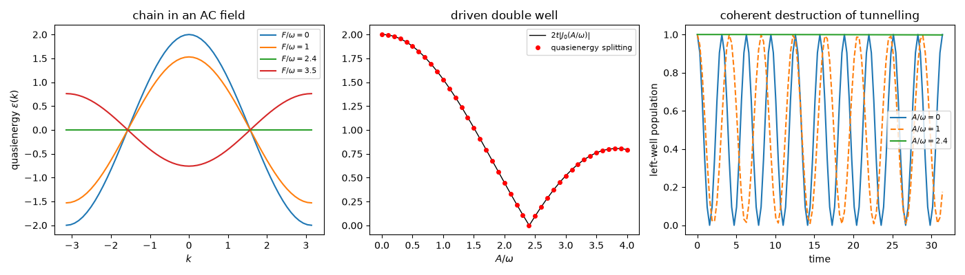
Largest deviation from 2t|J0(A/omega)|: 0.0048
Effective tunnelling at A/omega = 1: -0.7604 (-t J0(1) = -0.7652)
Lowest left-well population over 100 periods: 0.0000 (undriven), 0.9978 (A/omega = 2.405)