
Note
Go to the end to download the full example code.
The Optical Conductivity of Disordered Graphene, 45,000 Sites#
The Kubo-Greenwood formula gives the absorptive part of the optical conductivity as a joint density of occupied and empty states, weighted by the velocity between them:
In a crystal the trace is a sum over the Brillouin zone
(tbkit.optics.optical_conductivity()); in a disordered sample
there is no Brillouin zone. The kernel polynomial method expands both
deltas in Chebyshev polynomials, so that the trace becomes two-index
moments \(\mu_{mn} = \mathrm{Tr}[v_x T_m(\tilde H) v_x T_n(\tilde H)]\),
computed with a few random vectors and serving every frequency
(tbkit.kpm.optical_conductivity(), KITE’s
conductivity_optical).
Here: a clean graphene torus of \(150\times150\) cells, which gives the universal absorption \(\sigma_0 = \frac{\pi}{4}\frac{e^2}{h}\) (spinless: \(e^2/4\hbar\) once spin is counted) and the Brillouin-zone result, and the same torus with Anderson disorder, which fills the Pauli-blocked window \(\omega < 2|\mu|\) of doped graphene and smears out the van Hove peak at \(\omega = 2t\).
import numpy as np
import matplotlib.pyplot as plt

import tbkit.kpm as kpm
import tbkit.lattices as lattices
import tbkit.optics as optics
from tbkit.kspace import KSpace

t = 1.
n = 150  # 150 x 150 cells, 45,000 sites
gra = KSpace(lattices.honeycomb())
gra.set_hopping([{'i': 0, 'j': 1, 'R': R, 't': t} for R in [(0, 0), (-1, 0), (0, -1)]])
area = n * n * optics.cell_area(gra)
vx, _ = gra.finite_velocity(n, periodic=True, sparse=True)
omega = np.linspace(0.1, 3.5, 69)


def torus(w, seed=0):
    ham = gra.finite_ham(n, periodic=True, sparse=True).tolil()
    ham.setdiag(np.random.default_rng(seed).uniform(-w / 2, w / 2, 2 * n * n))
    return ham.tocsr()


def sigma(ham, e_fermi=0.):
    return kpm.optical_conductivity(ham, vx, omega, e_fermi=e_fermi, n_moments=192, n_random=16,
                                    seed=1, area=area)
The clean torus: universal absorption#
For kernel width \(\ll\omega\ll t\) the Dirac cones absorb \(\pi/4\) (in units of \(e^2/h\)) whatever the frequency; the lattice adds a van Hove peak at \(\omega = 2t\), the transitions at M. The Brillouin-zone Kubo formula (Lorentzian broadening \(\eta = 0.04t\)) gives the same curve, except where the two broadenings differ: at small \(\omega\), around the peak and on its tail.
clean = sigma(torus(0.))
bz = optics.optical_conductivity(gra, omega, eta=0.04, nk=400).real
plateau = (omega > 0.25) & (omega < 0.6)
print('clean, 0.25 < w < 0.6: sigma / (pi/4) between {:.3f} and {:.3f}'.format(
      *(clean[plateau].min() / (np.pi / 4), clean[plateau].max() / (np.pi / 4))))
# the mean to 3%, every point to the 1/sqrt(R N) noise of the random trace
assert abs(clean[plateau].mean() / (np.pi / 4) - 1.) < 0.03
assert np.allclose(clean[plateau], np.pi / 4, rtol=0.08)
# the two broadenings (Jackson kernel, Lorentzian eta) differ at small w,
# around the van Hove peak and on its tail: compare in between
between = (omega > 0.25) & (omega < 1.7)
print('KPM vs Brillouin zone, 0.25 < w < 1.7: largest deviation {:.1%}'.format(
      np.max(np.abs(clean[between] / bz[between] - 1.))))
assert np.allclose(clean[between], bz[between], rtol=0.05)
smooth = np.abs(omega - 2 * t) > 0.2
assert abs(omega[np.argmax(clean)] - 2 * t) < 0.1
clean, 0.25 < w < 0.6: sigma / (pi/4) between 0.988 and 1.016
KPM vs Brillouin zone, 0.25 < w < 1.7: largest deviation 3.0%
Doping and disorder#
At \(\mu = 0.5t\) the transitions below \(2\mu\) are Pauli blocked: the clean absorption drops to (almost) zero there, the kernel only rounding the step. Disorder \(W = 2.5t\) gives the states a finite lifetime and opens absorption below \(2\mu\) (and a Drude peak at small \(\omega\)), and it flattens the van Hove peak.
mu = 0.5
clean_doped = sigma(torus(0.), mu)
dirty_doped = sigma(torus(2.5), mu)
blocked = (omega > 0.3) & (omega < 0.75)
print('w in the Pauli-blocked window: clean {:.3f}, disordered {:.3f} (units of pi/4)'.format(
      clean_doped[blocked].mean() / (np.pi / 4), dirty_doped[blocked].mean() / (np.pi / 4)))
assert np.all(clean_doped[blocked] < 0.1 * np.pi / 4)
assert dirty_doped[blocked].mean() > 3 * clean_doped[blocked].mean()
step = omega > 1.3
assert np.allclose(clean_doped[step & smooth], clean[step & smooth], rtol=0.08)  # above 2 mu: undoped
print('van Hove peak: {:.2f} (clean), {:.2f} (disordered)'.format(clean_doped.max(), dirty_doped.max()))
assert dirty_doped.max() < 0.8 * clean_doped.max()

fig, ax = plt.subplots(figsize=(6.5, 4))
ax.plot(omega, bz / (np.pi / 4), color='0.6', lw=4, label=r'Brillouin zone, $\mu = 0$')
ax.plot(omega, clean / (np.pi / 4), 'b', label=r'KPM, $\mu = 0$')
ax.plot(omega, clean_doped / (np.pi / 4), 'g', label=r'KPM, $\mu = 0.5t$')
ax.plot(omega, dirty_doped / (np.pi / 4), 'r', label=r'KPM, $\mu = 0.5t$, $W = 2.5t$')
ax.axhline(1., color='k', ls='--', lw=1)
ax.set_xlabel(r'$\hbar\omega/t$')
ax.set_ylabel(r'$\mathrm{Re}\,\sigma_{xx}\,/\,\sigma_0$')
ax.set_ylim(0, None)
ax.legend(fontsize=9)
ax.set_title('Optical conductivity, 45,000 sites')
fig.set_layout_engine('tight')
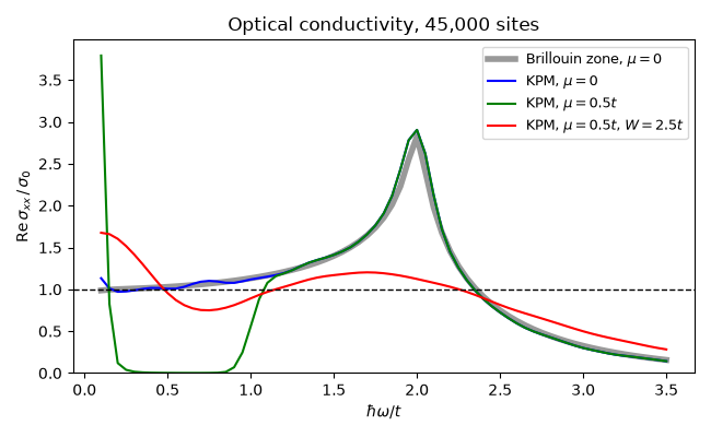
w in the Pauli-blocked window: clean 0.003, disordered 0.939 (units of pi/4)
van Hove peak: 2.98 (clean), 1.32 (disordered)
Total running time of the script: (0 minutes 25.473 seconds)