
Note
Go to the end to download the full example code.
The Spectral Function of Disordered Graphene, 28,800 Sites#
Photoemission (ARPES) measures the spectral function
\(A(\mathbf{k}, E)\): how much of a plane wave of momentum
\(\mathbf{k}\) lives at energy \(E\). In a crystal it is peaked
on the bands; disorder gives the quasiparticles a finite lifetime, which
broadens the peaks, and shifts them. Band unfolding
(tbkit.moire.spectral_function()) gets it from the eigenstates of
a supercell, which caps the sample at a few thousand orbitals. The kernel
polynomial method needs none: with one plane wave per sublattice o,
each k-point costs one Chebyshev recursion per sublattice, like a local
density of states (tbkit.kpm.spectral_function(), what KITE calls
arpes).
Here: the exact check against band unfolding on a small disordered supercell, then \(A(\mathbf{k}, E)\) along \(\Gamma\)-M-K-\(\Gamma\) of a graphene torus of \(120\times120\) cells with Anderson disorder.
import numpy as np
import matplotlib.pyplot as plt
from scipy.integrate import trapezoid

import tbkit.kpm as kpm
import tbkit.lattices as lattices
import tbkit.moire as moire
from tbkit.kspace import KSpace

t = 1.
gra = KSpace(lattices.honeycomb())
gra.set_hopping([{'i': 0, 'j': 1, 'R': R, 't': t} for R in [(0, 0), (-1, 0), (0, -1)]])
a_vec = np.array(gra.lat.prim_vec)[:, :2]
b_vec = 2 * np.pi * np.linalg.inv(a_vec).T  # reciprocal vectors (rows)
tau = gra.orbital_positions()[:, :2]


def torus(n, w, seed=0):
    '''The n x n graphene torus with box disorder of width w, and its row positions.'''
    ham = gra.finite_ham(n, periodic=True, sparse=True).tolil()
    ham.setdiag(np.random.default_rng(seed).uniform(-w / 2, w / 2, 2 * n * n))
    cells = np.array([(n1, n2) for n2 in range(n) for n1 in range(n)]) @ a_vec
    return ham.tocsr(), np.repeat(cells, 2, axis=0) + np.tile(tau, (n * n, 1))
Against band unfolding#
A \(6\times6\) supercell with random onsite energies, at
\(\Gamma\) of its own Brillouin zone, is the \(6\times6\)
torus. On the torus’s k-mesh the KPM spectral function equals the
unfolded weights \(W_J(\mathbf{k})\) of tbkit.moire.unfold(),
each level broadened by the same Chebyshev series.
n_sc = 6
sc = moire.supercell(gra, [[n_sc, 0], [0, n_sc]])
sc.onsite = np.random.default_rng(1).uniform(-0.5, 0.5, sc.norb)
ham_sc = sc._bloch_ham(np.zeros((1, 2)))[0]
pos_sc = np.repeat(sc.cells[:, :2], 2, axis=0) + np.tile(tau, (n_sc * n_sc, 1))
k_check = np.array([[0., 0.], [0.5, 0.], [2 / 3, 1 / 3], [1 / 3, 1 / 6]]) @ b_vec
e_check, a_kpm = kpm.spectral_function(ham_sc, pos_sc, k_check, np.tile([0, 1], n_sc * n_sc), 96)
en, weights = moire.unfold(sc, k_check)
bounds = kpm.spectral_bounds(ham_sc)
a_unf = np.array([weights[i] @ np.array([kpm.dos_from_levels([e], 96, bounds, e_check) for e in en[i]])
                      for i in range(len(k_check))])
gap = np.abs(a_kpm - a_unf).max()
print('KPM vs band unfolding, 72 orbitals: largest difference {:.1e}'.format(gap))
assert gap < 1e-9
KPM vs band unfolding, 72 orbitals: largest difference 2.7e-12
28,800 sites#
The path \(\Gamma\)-M-K-\(\Gamma\) through points of the \(120\times120\) mesh (in units of the reciprocal vectors: M = (1/2, 0), K = (2/3, 1/3)), clean and with box disorder of width \(W = 2t\). Each spectral function integrates to 2, the number of sublattices.
n = 120
path = ([(i, 0) for i in range(0, 60)] + [(60 + i, 2 * i) for i in range(0, 20)]
        + [(80 - 2 * i, 40 - i) for i in range(0, 41)])
frac = np.array(path) / n
k_path = frac @ b_vec
e_grid = np.linspace(-3.9, 3.9, 391)
spectra = {}
for w in (0., 2.):
    ham, pos = torus(n, w)
    _, spectra[w] = kpm.spectral_function(ham, pos, k_path, np.tile(['a', 'b'], n * n), 384, e_grid,
                                                bounds=(-4., 4.))
    print('W = {}: {} sites, integral of A between {:.3f} and {:.3f}'.format(
          w, ham.shape[0], *np.sort(trapezoid(spectra[w], e_grid, axis=1))[[0, -1]]))
    assert np.allclose(trapezoid(spectra[w], e_grid, axis=1), 2., atol=0.02)
bands = np.linalg.eigvalsh(gra._bloch_ham(k_path))
W = 0.0: 28800 sites, integral of A between 2.000 and 2.000
W = 2.0: 28800 sites, integral of A between 2.000 and 2.000
The clean peaks sit on the bands; disorder lowers and widens them (a finite lifetime) – most near the van Hove energy \(|E| = t\) at M, where the density of states to scatter into is largest.
upper = e_grid > 0
peak_clean = e_grid[upper][np.argmax(spectra[0.][:, upper], axis=1)]
assert np.allclose(peak_clean[1:], bands[1:, 1], atol=0.04)  # (at Gamma, E = 3t is the band edge)


def width(spec):
    '''Full width at half maximum of the upper peak.'''
    s = spec[upper]
    above = e_grid[upper][s > s.max() / 2]
    return above.max() - above.min()


i_m = 60
w_clean, w_dirty = width(spectra[0.][i_m]), width(spectra[2.][i_m])
print('Peak at M: width {:.3f} (clean, the kernel), {:.3f} (W = 2t)'.format(w_clean, w_dirty))
assert w_dirty > 2 * w_clean
assert spectra[2.][i_m].max() < 0.5 * spectra[0.][i_m].max()

fig, axes = plt.subplots(1, 2, figsize=(10, 4.2), sharey=True)
ticks = [0, 60, 80, len(path) - 1]
for axis, w in zip(axes, (0., 2.)):
    axis.imshow(spectra[w].T ** 0.5, origin='lower', aspect='auto', cmap='magma',
                    extent=(0, len(path) - 1, e_grid[0], e_grid[-1]))
    axis.plot(bands, color='c', lw=0.6, ls='--')
    axis.set_xticks(ticks)
    axis.set_xticklabels([r'$\Gamma$', 'M', 'K', r'$\Gamma$'])
    axis.set_title('clean' if w == 0 else 'disorder $W = {:g}t$'.format(w))
axes[0].set_ylabel('$E/t$')
fig.suptitle(r'$A(\mathbf{k}, E)$ of a graphene torus, 28,800 sites (KPM)')
fig.set_layout_engine('tight')
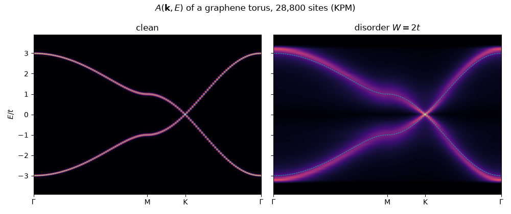
Peak at M: width 0.040 (clean, the kernel), 0.540 (W = 2t)
Total running time of the script: (0 minutes 40.021 seconds)