Peukert’s law: battery capacity falls at high discharge rates

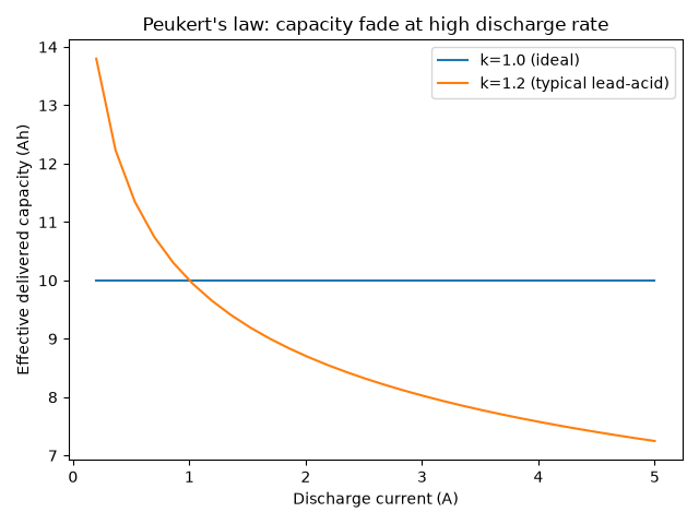
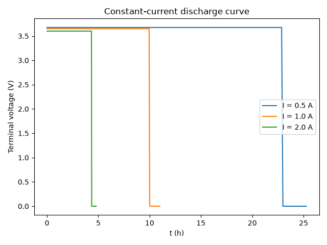
Peukert’s 1897 power law, \(t = C_p/I^k\), says a lead-acid battery discharged faster delivers less total charge. Using effective_capacity(), this example compares the ideal Peukert exponent k=1 (same capacity at every rate) with a realistic k=1.2, then draws discharge curves from ConstantCurrentBattery (a deliberately simplified model; see its docstring) whose runtimes shrink faster than 1/I.

import matplotlib.pyplot as plt
import numpy as np

from chemistrykit.electrochem.systems.battery import ConstantCurrentBattery, effective_capacity
from chemistrykit.electrochem.visualizers.electrochem_plots import plot_discharge_curve

Ideal (k=1) vs. real (k=1.2) Peukert-law effective capacity vs. rate.

currents = np.linspace(0.2, 5.0, 30)
C_p = 10.0
C_eff_ideal = effective_capacity(C_p, currents, k=1.0)
C_eff_real = effective_capacity(C_p, currents, k=1.2)

fig, ax = plt.subplots()
ax.plot(currents, C_eff_ideal, label="k=1.0 (ideal)")
ax.plot(currents, C_eff_real, label="k=1.2 (typical lead-acid)")
ax.set_xlabel("Discharge current (A)")
ax.set_ylabel("Effective delivered capacity (Ah)")
ax.set_title("Peukert's law: capacity fade at high discharge rate")
ax.legend()
fig.tight_layout()

Discharge curves at a few different constant currents, all from the same Peukert capacity constant.

fig2, ax2 = plt.subplots()
for current in (0.5, 1.0, 2.0):
    battery = ConstantCurrentBattery(capacity_peukert=C_p, current=current, v_nominal=3.7, internal_resistance=0.05, k=1.2)
    plot_discharge_curve(battery, ax=ax2, label=f"I = {current} A")
ax2.legend()
fig2.tight_layout()

plt.show()