Kohlrausch’s laws: independent migration and the square-root law

Kohlrausch found that the molar conductivity of a strong electrolyte falls linearly with \(\sqrt{c}\), \(\Lambda_m = \Lambda_m^\circ - K\sqrt{c}\), and that the infinite-dilution value \(\Lambda_m^\circ\) is a sum of independent ionic contributions. This example extrapolates noisy KCl data to infinite dilution with fit_kohlrausch_law(), and uses limiting_molar_conductivity() for his classic trick: the limiting conductivity of the weak acid acetic acid, which cannot be extrapolated, from three strong electrolytes.

import matplotlib.pyplot as plt
import numpy as np

from chemistrykit.electrochem.systems.conductivity import (
    fit_kohlrausch_law,
    kohlrausch_molar_conductivity,
    limiting_molar_conductivity,
)

Square-root law: synthetic KCl data (Lambda0 from the ionic table, K ~ 9.2e-3 S m^2 mol^-1 (mol/L)^-1/2) with 0.1% noise.

rng = np.random.default_rng(1875)
Lambda0_KCl = limiting_molar_conductivity({"K+": 1, "Cl-": 1})
c = np.linspace(1e-4, 1e-2, 12)
Lambda_meas = kohlrausch_molar_conductivity(c, Lambda0_KCl, 9.2e-3) * (1 + rng.normal(0.0, 1e-3, c.size))
fit = fit_kohlrausch_law(c, Lambda_meas)
print(f"KCl: table Lambda0 = {Lambda0_KCl * 1e4:.1f}, extrapolated = {fit.limiting_molar_conductivity * 1e4:.1f} S cm^2/mol")

fig, (ax1, ax2) = plt.subplots(1, 2, figsize=(10, 4))
x = np.linspace(0.0, 0.1, 50)
ax1.plot(np.sqrt(c), Lambda_meas * 1e4, "o", label="KCl data")
ax1.plot(x, (fit.limiting_molar_conductivity - fit.kohlrausch_coefficient * x) * 1e4, label="Kohlrausch fit")
ax1.set_xlabel(r"$\sqrt{c}$ (mol/L)$^{1/2}$")
ax1.set_ylabel(r"$\Lambda_m$ (S cm$^2$ mol$^{-1}$)")
ax1.set_title("Square-root law")
ax1.legend()

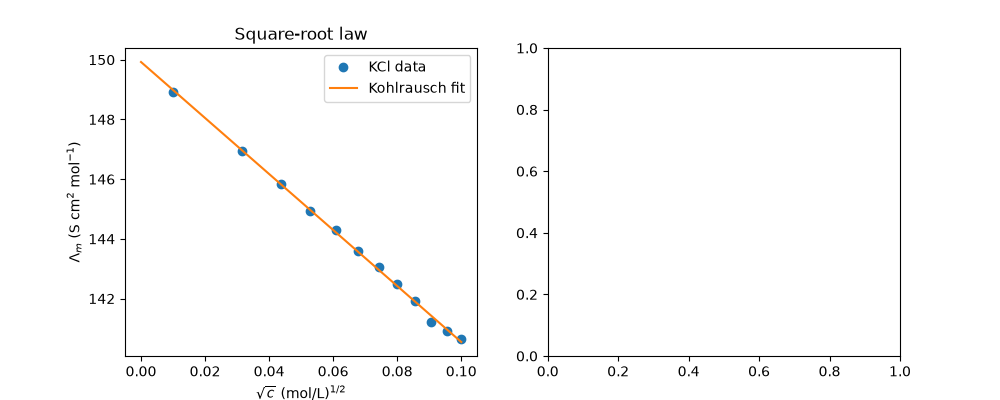
KCl: table Lambda0 = 149.8, extrapolated = 149.9 S cm^2/mol

<matplotlib.legend.Legend object at 0x1196916a0>

Independent migration: Lambda0(HAc) = Lambda0(HCl) + Lambda0(NaAc) - Lambda0(NaCl).

salts = {
    "HCl": {"H+": 1, "Cl-": 1},
    "NaAc": {"Na+": 1, "CH3COO-": 1},
    "NaCl": {"Na+": 1, "Cl-": 1},
}
values = {name: limiting_molar_conductivity(ions) for name, ions in salts.items()}
values["HAc"] = values["HCl"] + values["NaAc"] - values["NaCl"]
for name, v in values.items():
    print(f"Lambda0({name}) = {v * 1e4:.1f} S cm^2/mol")

ax2.bar(list(values), [v * 1e4 for v in values.values()], color=["gray", "gray", "gray", "crimson"])
ax2.set_ylabel(r"$\Lambda_m^\circ$ (S cm$^2$ mol$^{-1}$)")
ax2.set_title("HAc = HCl + NaAc - NaCl")
fig.tight_layout()
plt.show()

Lambda0(HCl) = 425.9 S cm^2/mol
Lambda0(NaAc) = 91.0 S cm^2/mol
Lambda0(NaCl) = 126.4 S cm^2/mol
Lambda0(HAc) = 390.5 S cm^2/mol