Grove’s gas battery: the hydrogen-oxygen fuel cell

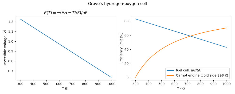
In 1839-1842 William Grove ran electrolysis backwards: hydrogen and oxygen over platinum electrodes in dilute acid recombined to produce a current. This example computes the reversible voltage of that cell two ways – from the standard potentials of the O2/H2O and H+/H2 couples and from \(\Delta G^\circ\) via reversible_cell_voltage() – its temperature dependence (reversible_cell_voltage_at_temperature()), and its thermodynamic efficiency limit \(\Delta G/\Delta H\) (fuel_cell_efficiency_limit()) compared with the Carnot limit of a heat engine.

import matplotlib.pyplot as plt
import numpy as np

from chemistrykit.electrochem.systems.fuel_cell import (
    fuel_cell_efficiency_limit,
    reversible_cell_voltage,
    reversible_cell_voltage_at_temperature,
)
from chemistrykit.electrochem.systems.standard_potentials import standard_cell_potential

# H2 + 1/2 O2 -> H2O(l) at 298.15 K (standard thermochemical data).
dG, dH, dS, n = -237.13e3, -285.83e3, -163.3, 2

E_table = standard_cell_potential("O2/H2O", "H+/H2")
E_gibbs = reversible_cell_voltage(dG, n)
print(f"From standard potentials: {E_table:.3f} V; from Delta G: {E_gibbs:.3f} V")
print(f"Maximum efficiency Delta G / Delta H = {fuel_cell_efficiency_limit(dG, dH):.1%}")

From standard potentials: 1.230 V; from Delta G: 1.229 V
Maximum efficiency Delta G / Delta H = 83.0%

Reversible voltage and efficiency limit vs. temperature, compared with a Carnot engine rejecting heat at 298 K.

T = np.linspace(300.0, 1000.0, 100)
E_T = reversible_cell_voltage_at_temperature(dH, dS, n, T)
eff_fc = fuel_cell_efficiency_limit(dH - T * dS, dH)
eff_carnot = 1.0 - 298.15 / T

fig, (ax1, ax2) = plt.subplots(1, 2, figsize=(10, 4))
ax1.plot(T, E_T)
ax1.set_xlabel("T (K)")
ax1.set_ylabel("Reversible voltage (V)")
ax1.set_title(r"$E(T) = -(\Delta H - T\Delta S)/nF$")
ax2.plot(T, eff_fc * 100, label=r"fuel cell, $\Delta G/\Delta H$")
ax2.plot(T, eff_carnot * 100, label="Carnot engine (cold side 298 K)")
ax2.set_xlabel("T (K)")
ax2.set_ylabel("Efficiency limit (%)")
ax2.legend()
fig.suptitle("Grove's hydrogen-oxygen cell")
fig.tight_layout()
plt.show()