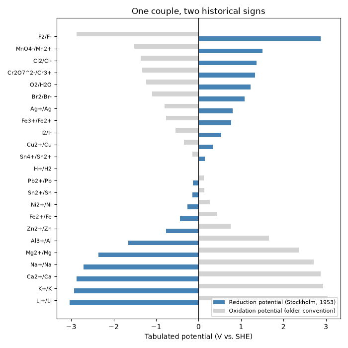
The 1953 Stockholm convention: electrode potentials are reduction potentials

Before IUPAC’s 1953 Stockholm meeting, one tradition tabulated oxidation potentials and another reduction potentials, so the same couple appeared with opposite signs in different books. This example shows both conventions for the table in STANDARD_REDUCTION_POTENTIALS (which follows Stockholm), and shows that the cathode-minus-anode rule of cell_potential() only gives the right cell voltage and spontaneity when both half-reactions use the agreed reduction convention.

import matplotlib.pyplot as plt
import numpy as np

from chemistrykit.electrochem.systems.standard_potentials import STANDARD_REDUCTION_POTENTIALS as T
from chemistrykit.electrochem.systems.standard_potentials import cell_potential, is_spontaneous

Correct usage: both values are Stockholm reduction potentials.

E_ok = cell_potential(T["Ag+/Ag"], T["Cu2+/Cu"])
print(f"Ag+/Ag cathode, Cu anode (both reduction potentials): E = {E_ok:+.2f} V, spontaneous = {is_spontaneous(E_ok)}")

Ag+/Ag cathode, Cu anode (both reduction potentials): E = +0.46 V, spontaneous = True

The historical pitfall: taking the anode value from an oxidation-potential table (sign flipped) and subtracting it gives nonsense.

E_mixed = T["Ag+/Ag"].E_standard - (-T["Cu2+/Cu"].E_standard)
print(f"Same cell with a mixed-convention anode value: E = {E_mixed:+.2f} V (wrong; measured 0.46 V)")

Same cell with a mixed-convention anode value: E = +1.14 V (wrong; measured 0.46 V)

The whole table in both conventions: the oxidation-potential column is the mirror image of the Stockholm (reduction) column.

names = list(T)
E_red = np.array([T[name].E_standard for name in names])
order = np.argsort(E_red)
y = np.arange(len(names))

fig, ax = plt.subplots(figsize=(7, 7))
ax.barh(y - 0.2, E_red[order], height=0.4, color="steelblue", label="Reduction potential (Stockholm, 1953)")
ax.barh(y + 0.2, -E_red[order], height=0.4, color="lightgray", label="Oxidation potential (older convention)")
ax.set_yticks(y)
ax.set_yticklabels([names[i] for i in order], fontsize=8)
ax.axvline(0.0, color="black", linewidth=0.8)
ax.set_xlabel("Tabulated potential (V vs. SHE)")
ax.set_title("One couple, two historical signs")
ax.legend(fontsize=8, loc="lower right")
fig.tight_layout()
plt.show()