Recovering an activation energy from an Arrhenius plot

Synthetic rate-constant-vs-temperature data is generated from a known activation energy \(E_a\) and pre-exponential factor \(A\), then fit_arrhenius() recovers both parameters back out via the classic Arrhenius-plot linearization (\(\ln k\) vs. \(1/T\)).

import matplotlib.pyplot as plt
import numpy as np

from chemistrykit.kinetics.systems.arrhenius import arrhenius_rate_constant, fit_arrhenius
from chemistrykit.kinetics.visualizers.kinetics_plots import plot_arrhenius

A_true, Ea_true = 4.2e12, 65_000.0  # J/mol
T = np.linspace(280.0, 360.0, 9)

rng = np.random.default_rng(0)
k_exact = arrhenius_rate_constant(A=A_true, Ea=Ea_true, T=T)
# A small amount of multiplicative noise, as a real kinetics measurement would have.
k_noisy = k_exact * (1.0 + rng.normal(0.0, 0.02, size=T.shape))

fit = fit_arrhenius(T, k_noisy)
print(f"true:   Ea={Ea_true:.0f} J/mol, A={A_true:.3e}")
print(f"fitted: Ea={fit.Ea:.0f} J/mol, A={fit.A:.3e}, R^2={fit.r_squared:.5f}")

true:   Ea=65000 J/mol, A=4.200e+12
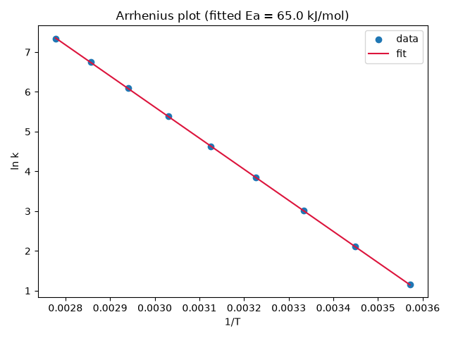
fitted: Ea=65046 J/mol, A=4.293e+12, R^2=0.99996

The Arrhenius plot: a straight line of slope \(-E_a/R\).

ax = plot_arrhenius(T, k_noisy, fit=fit)
ax.set_title(f"Arrhenius plot (fitted Ea = {fit.Ea / 1000:.1f} kJ/mol)")
plt.tight_layout()
plt.show()