Lineweaver and Burk’s double-reciprocal plot

Lineweaver and Burk (1934) inverted the Michaelis-Menten equation into a straight line, \(1/v = (K_m/V_{max})(1/[S]) + 1/V_{max}\), so \(V_{max}\) and \(K_m\) could be read off the intercept and slope. fit_lineweaver_burk() does exactly that fit on noisy initial-rate data. The second panel shows the method’s well-known weakness: the same small relative noise becomes a large scatter at the low-[S] (large \(1/[S]\)) end, which dominates the fitted line.

import matplotlib.pyplot as plt
import numpy as np

from chemistrykit.kinetics.systems.enzyme import fit_lineweaver_burk, michaelis_menten_rate
from chemistrykit.kinetics.visualizers.kinetics_plots import plot_lineweaver_burk

Vmax, Km = 10.0, 2.0
S_samples = np.array([0.5, 1.0, 2.0, 4.0, 8.0, 16.0])

rng = np.random.default_rng(1)
v_exact = michaelis_menten_rate(S_samples, Vmax, Km)
v_noisy = v_exact * (1.0 + rng.normal(0.0, 0.03, size=S_samples.shape))
fit = fit_lineweaver_burk(S_samples, v_noisy)
print(f"true:   Vmax={Vmax}, Km={Km}")
print(f"fitted: Vmax={fit.Vmax:.3f}, Km={fit.Km:.3f}, R^2={fit.r_squared:.5f}")

fig, axes = plt.subplots(1, 2, figsize=(11, 4.5))
plot_lineweaver_burk(S_samples, v_noisy, fit=fit, ax=axes[0])
axes[0].set_title(f"Lineweaver-Burk fit: Vmax={fit.Vmax:.2f}, Km={fit.Km:.2f}")

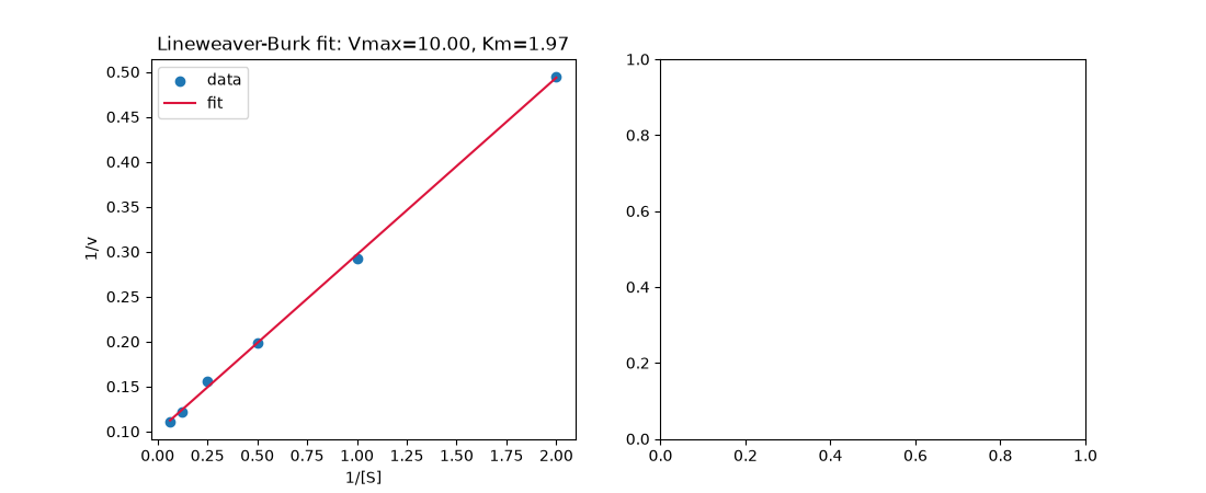
true:   Vmax=10.0, Km=2.0
fitted: Vmax=10.004, Km=1.968, R^2=0.99929

Text(0.5, 1.0, 'Lineweaver-Burk fit: Vmax=10.00, Km=1.97')

Error distortion: repeat the “experiment” many times with 3% noise and look at the spread of each point in reciprocal coordinates.

trials = np.array([1.0 / (v_exact * (1.0 + rng.normal(0.0, 0.03, size=S_samples.shape))) for _ in range(200)])
axes[1].errorbar(1.0 / S_samples, trials.mean(axis=0), yerr=trials.std(axis=0), fmt="o", capsize=4, color="steelblue")
axes[1].set_xlabel("1/[S]")
axes[1].set_ylabel("1/v  (mean +/- std over 200 trials)")
axes[1].set_title("Same 3% noise, very unequal reciprocal error bars")
for inv_s, spread in zip(1.0 / S_samples, trials.std(axis=0)):
    print(f"1/[S] = {inv_s:5.3f}: std of 1/v = {spread:.4f}")

fig.tight_layout()
plt.show()

1/[S] = 2.000: std of 1/v = 0.0152
1/[S] = 1.000: std of 1/v = 0.0090
1/[S] = 0.500: std of 1/v = 0.0059
1/[S] = 0.250: std of 1/v = 0.0044
1/[S] = 0.125: std of 1/v = 0.0036
1/[S] = 0.062: std of 1/v = 0.0035