van’t Hoff’s reaction orders: zero-, first-, and second-order rate laws

van’t Hoff (1884) classified reactions by the order \(n\) of their rate law \(-d[A]/dt = k[A]^n\). The three textbook cases – ZeroOrder, FirstOrder, and SecondOrder – all started from the same initial concentration and with rate constants chosen to give the same half-life, so the different curvature (linear, exponential, hyperbolic) is the only thing distinguishing them. First order is the only one whose half-life doesn’t depend on the starting concentration; the plot below marks all three half-lives to make that concrete.

import matplotlib.pyplot as plt
import numpy as np

from chemistrykit.kinetics.systems.rate_laws import FirstOrder, SecondOrder, ZeroOrder

C0 = 1.0
t_half_target = 5.0

zero = ZeroOrder(k=C0 / (2.0 * t_half_target), C0=C0)
first = FirstOrder(k=np.log(2.0) / t_half_target, C0=C0)
second = SecondOrder(k=1.0 / (t_half_target * C0), C0=C0)

t = np.linspace(0.0, 20.0, 400)

fig, ax = plt.subplots(figsize=(7, 5))
for law, label, color in [(zero, "zero order", "steelblue"), (first, "first order", "darkorange"), (second, "second order", "seagreen")]:
    ax.plot(t, np.clip(law.concentration(t), 0.0, None), label=f"{label} (t_1/2={law.half_life():.2f})", color=color)
    ax.axvline(law.half_life(), color=color, linestyle=":", alpha=0.5)

ax.axhline(C0 / 2.0, color="gray", linestyle="--", linewidth=0.8, label="[A]_0 / 2")
ax.set_xlabel("t")
ax.set_ylabel("[A]")
ax.set_title("Same half-life, three different rate laws")
ax.legend()
fig.tight_layout()

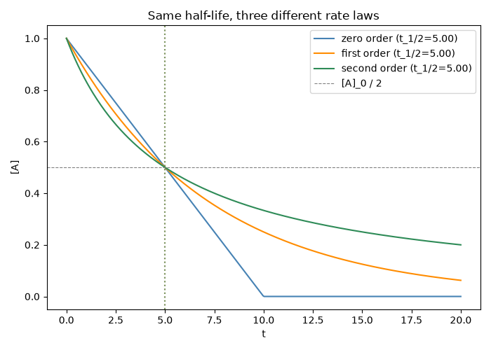
All three curves cross [A]_0/2 at their respective half-life by construction. The zero-order law is the only one that reaches exactly zero (and stays there – the model doesn’t allow negative concentration), while first- and second-order decay approach zero only asymptotically.

for law, label in [(zero, "zero"), (first, "first"), (second, "second")]:
    print(f"{label}-order: [A](t_1/2) = {law.concentration(law.half_life()):.6f} (expected {C0 / 2.0})")

zero-order: [A](t_1/2) = 0.500000 (expected 0.5)
first-order: [A](t_1/2) = 0.500000 (expected 0.5)
second-order: [A](t_1/2) = 0.500000 (expected 0.5)

van’t Hoff’s differential method: measure the initial rate at several starting concentrations. Since \(\log v_0 = \log k + n\log[A]_0\), the slope of a log-log plot of initial rate against initial concentration reads off the order \(n\) directly.

C0_values = np.array([0.25, 0.5, 1.0, 2.0, 4.0])
fig2, ax2 = plt.subplots(figsize=(7, 5))
for cls, k, label, color in [
    (ZeroOrder, 0.1, "zero order", "steelblue"),
    (FirstOrder, 0.1, "first order", "darkorange"),
    (SecondOrder, 0.1, "second order", "seagreen"),
]:
    v0 = np.array([cls(k=k, C0=c).rate(0.0) for c in C0_values])
    n_fit = np.polyfit(np.log(C0_values), np.log(v0), 1)[0]
    ax2.loglog(C0_values, v0, "o-", color=color, label=f"{label}: fitted slope n = {n_fit:.2f}")
    print(f"{label}: order from log-log slope = {n_fit:.3f}")
ax2.set_xlabel("[A]_0")
ax2.set_ylabel("initial rate v_0")
ax2.set_title("Reading off the reaction order from initial rates")
ax2.legend()
fig2.tight_layout()

plt.show()

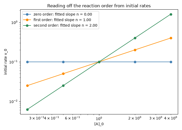
zero order: order from log-log slope = 0.000
first order: order from log-log slope = 1.000
second order: order from log-log slope = 2.000