Trautz-Lewis collision theory: rate constants from molecular collisions

Trautz (1916) and Lewis (1918) computed a gas-phase rate constant as the number of collisions per unit time times the Boltzmann fraction with enough energy,

\[k = P\,\sigma \sqrt{\frac{8k_BT}{\pi\mu}}\,N_A\,e^{-E_a/RT},\]

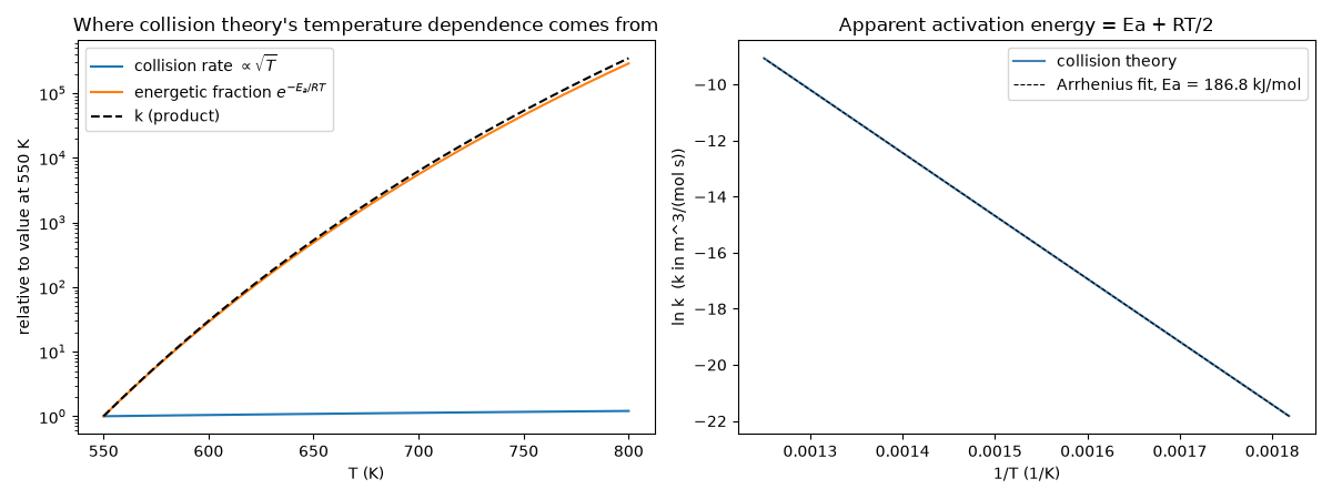
evaluated by collision_theory_rate_constant(). The left panel shows its two ingredients – the collision rate grows only as \(\sqrt{T}\), while the energetic fraction grows exponentially. The right panel shows that an Arrhenius fit to collision-theory rate constants returns \(E_a + RT/2\), because the prefactor itself depends weakly on temperature. Lewis’s test case was \(2\,\text{HI} \to \text{H}_2 + \text{I}_2\); the molecular parameters below are illustrative values of that order.

collision rate constant at 700 K: 2.078e-03 L/(mol s)
Arrhenius fit: Ea_app = 186.75 kJ/mol; Ea + RT/2 = 186.77 kJ/mol

import matplotlib.pyplot as plt
import numpy as np

from chemistrykit.constants import ATOMIC_MASS_UNIT, R
from chemistrykit.kinetics.systems.arrhenius import fit_arrhenius
from chemistrykit.kinetics.systems.rate_theory import collision_theory_rate_constant

m_HI = 127.91 * ATOMIC_MASS_UNIT
mu = m_HI / 2.0  # identical collision partners
d = 3.5e-10  # collision diameter, m (illustrative)
sigma = np.pi * d**2
Ea = 184e3  # J/mol, of the order of the HI decomposition barrier

T = np.linspace(550.0, 800.0, 60)
collision_part = collision_theory_rate_constant(T, sigma, mu)  # every collision reacts
k = collision_theory_rate_constant(T, sigma, mu, Ea=Ea)

fig, axes = plt.subplots(1, 2, figsize=(12, 4.5))
axes[0].semilogy(T, collision_part / collision_part[0], label=r"collision rate $\propto\sqrt{T}$")
axes[0].semilogy(T, np.exp(-Ea / (R * T)) / np.exp(-Ea / (R * T[0])), label=r"energetic fraction $e^{-E_a/RT}$")
axes[0].semilogy(T, k / k[0], "k--", label="k (product)")
axes[0].set_xlabel("T (K)")
axes[0].set_ylabel("relative to value at 550 K")
axes[0].set_title("Where collision theory's temperature dependence comes from")
axes[0].legend()

fit = fit_arrhenius(T, k)
T_mid = 1.0 / np.mean(1.0 / T)
print(f"collision rate constant at 700 K: {collision_theory_rate_constant(700.0, sigma, mu, Ea=Ea) * 1000:.3e} L/(mol s)")
print(f"Arrhenius fit: Ea_app = {fit.Ea / 1000:.2f} kJ/mol; Ea + RT/2 = {(Ea + 0.5 * R * T_mid) / 1000:.2f} kJ/mol")

axes[1].plot(1.0 / T, np.log(k), color="steelblue", label="collision theory")
axes[1].plot(1.0 / T, np.log(fit.predict(T)), "k--", linewidth=0.8, label=f"Arrhenius fit, Ea = {fit.Ea / 1000:.1f} kJ/mol")
axes[1].set_xlabel("1/T (1/K)")
axes[1].set_ylabel("ln k  (k in m^3/(mol s))")
axes[1].set_title("Apparent activation energy = Ea + RT/2")
axes[1].legend()

fig.tight_layout()
plt.show()