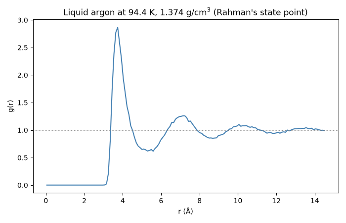
Rahman’s liquid argon: g(r) of a Lennard-Jones liquid in real units

Rahman’s 1964 simulation followed 864 argon atoms interacting through a Lennard-Jones potential with \(\epsilon/k_B = 120\ \text{K}\) and \(\sigma = 3.4\ \text{\AA}\), at \(T = 94.4\ \text{K}\) and a mass density of \(1.374\ \text{g/cm}^3\) – liquid argon just above its triple point. Here the same state point is simulated with LJFluid (512 atoms, reduced units), and the radial distribution function (radial_distribution_function()) is converted back to ångströms, as Rahman compared it with neutron- and X-ray-scattering data on real liquid argon.

import matplotlib.pyplot as plt
import numpy as np

from chemistrykit.constants import NA
from chemistrykit.md.systems.lj_fluid import LJFluid
from chemistrykit.md.systems.thermostats import VelocityRescalingThermostat

epsilon_over_k, sigma_A, molar_mass = 120.0, 3.4, 39.948  # K, angstrom, g/mol (Rahman's argon)
T_kelvin, rho_mass = 94.4, 1.374  # K, g/cm^3

rho_reduced = rho_mass / molar_mass * NA * (sigma_A * 1e-8) ** 3
T_reduced = T_kelvin / epsilon_over_k
print(f"reduced density rho* = {rho_reduced:.3f}, reduced temperature T* = {T_reduced:.3f}")

fluid = LJFluid.from_lattice(n_per_side=8, density=rho_reduced, temperature=T_reduced, cutoff=2.5, rng=0)
# melt the starting lattice and equilibrate at Rahman's temperature, then run NVE
fluid.run(dt=0.005, n_steps=3000, thermostat=VelocityRescalingThermostat(T_reduced, interval=10), sample_every=3000)
result = fluid.run(dt=0.005, n_steps=2000, sample_every=100)

g_frames = [fluid.radial_distribution_function(n_bins=150, positions=p)[1] for p in result.positions]
r, _ = fluid.radial_distribution_function(n_bins=150)
g = np.mean(g_frames, axis=0)
r_A = r * sigma_A

fig, ax = plt.subplots(figsize=(7, 4.5))
ax.plot(r_A, g, color="steelblue")
ax.axhline(1.0, color="gray", linestyle=":", linewidth=0.8)
ax.set_xlabel(r"r ($\mathrm{\AA}$)")
ax.set_ylabel("g(r)")
ax.set_title(f"Liquid argon at {T_kelvin} K, {rho_mass} g/cm$^3$ (Rahman's state point)")
fig.tight_layout()

reduced density rho* = 0.814, reduced temperature T* = 0.787

The first peak sits near 3.7 Å and the structure dies away after two or three coordination shells – the liquid signature Rahman compared with experiment. Integrating \(4\pi\rho r^2 g(r)\) out to the first minimum counts the nearest neighbors of an atom: a little more than a dozen, a nearly close-packed first shell like that of the crystal the liquid freezes into:

i_peak = int(np.argmax(g))
i_min = i_peak + int(np.argmin(g[i_peak : i_peak + 40]))
dr = r[1] - r[0]
coordination = float(np.sum(4.0 * np.pi * rho_reduced * r[:i_min] ** 2 * g[:i_min]) * dr)
print(f"first peak at r = {r_A[i_peak]:.2f} angstrom, first minimum at {r_A[i_min]:.2f} angstrom")
print(f"coordination number (first shell): {coordination:.1f}")

plt.show()

first peak at r = 3.74 angstrom, first minimum at 5.58 angstrom
coordination number (first shell): 13.6