Einstein’s diffusion law: mean-squared displacement grows linearly in time

Einstein’s 1905 analysis of Brownian motion showed that a particle performing a random walk wanders off, on average, not in proportion to time but to its square root: the mean-squared displacement grows linearly,

\[\langle |\vec r(t) - \vec r(0)|^2 \rangle = 6Dt \quad (t\to\infty,\ 3\text{D}),\]

with the self-diffusion coefficient \(D\) as the slope. In a simulated Lennard-Jones liquid every atom performs such a random walk, kicked about by its neighbors. This example unwraps the periodic trajectory (unwrap_trajectory()), computes the time-origin-averaged mean-squared displacement (mean_squared_displacement()), and reads \(D\) from the linear regime (einstein_diffusion_coefficient()).

import matplotlib.pyplot as plt
import numpy as np

from chemistrykit.md.systems.lj_fluid import LJFluid
from chemistrykit.md.systems.thermostats import VelocityRescalingThermostat
from chemistrykit.md.systems.transport import einstein_diffusion_coefficient, mean_squared_displacement

T, dt, sample_every = 1.0, 0.005, 4
fluid = LJFluid.from_lattice(n_per_side=6, density=0.7, temperature=T, cutoff=2.5, rng=0)
fluid.run(dt=dt, n_steps=2000, thermostat=VelocityRescalingThermostat(T, interval=10), sample_every=2000)
result = fluid.run(dt=dt, n_steps=4000, sample_every=sample_every)

max_lag = 500
msd = mean_squared_displacement(result.positions, box_length=result.box_length, max_lag=max_lag)
lag_t = np.arange(max_lag + 1) * dt * sample_every
D = einstein_diffusion_coefficient(lag_t, msd, fit_from=2.0)

fig, axes = plt.subplots(1, 2, figsize=(11, 4.5))
axes[0].plot(lag_t, msd, color="steelblue", label="simulated MSD")
axes[0].plot(lag_t, 6.0 * D * lag_t, color="black", linestyle="--", label=f"6Dt, D = {D:.3f}")
axes[0].set_xlabel("t")
axes[0].set_ylabel(r"$\langle|\Delta \vec r|^2\rangle$")
axes[0].set_title("Mean-squared displacement")
axes[0].legend()

axes[1].loglog(lag_t[1:], msd[1:], color="steelblue", label="simulated MSD")
v2 = 3.0 * T  # <v^2> = 3 k_B T / m
axes[1].loglog(lag_t[1:40], v2 * lag_t[1:40] ** 2, color="gray", linestyle=":", label=r"ballistic $\langle v^2\rangle t^2$")
axes[1].loglog(lag_t[40:], 6.0 * D * lag_t[40:], color="black", linestyle="--", label="diffusive 6Dt")
axes[1].set_xlabel("t")
axes[1].set_title("Log-log: ballistic, then diffusive")
axes[1].legend()
fig.tight_layout()

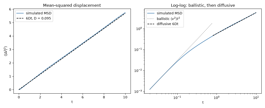
At very short times an atom simply flies freely (MSD grows as \(t^2\)); after a few collisions its motion becomes a random walk and the MSD settles onto Einstein’s straight line:

print(f"self-diffusion coefficient (reduced units): D = {D:.4f}")

plt.show()

self-diffusion coefficient (reduced units): D = 0.0949