Buckingham vs. Lennard-Jones: exponential repulsion and its inner turnover

The Buckingham (exp-6) potential replaces the Lennard-Jones \(r^{-12}\) repulsive wall with an exponential – closer to the true quantum-mechanical electron-overlap repulsion – while keeping the same \(r^{-6}\) dispersion attraction. Matched to a Lennard-Jones potential’s well depth, position, and long-range tail, the two agree closely everywhere near and beyond the minimum. But the exponential repulsion is eventually overwhelmed by the unbounded \(-C/r^6\) attractive term at short enough range, so the Buckingham potential has a second, spurious turnover well inside the true minimum: past that point it falls back toward \(-\infty\) as \(r\to0\) instead of diverging to \(+\infty\) the way Lennard-Jones’s pure \(r^{-12}\) repulsion does.

import matplotlib.pyplot as plt
import numpy as np

from chemistrykit.md.systems.lj_fluid import LennardJones
from chemistrykit.md.systems.pair_potentials import Buckingham

lj = LennardJones(epsilon=1.0, sigma=1.0)

# Match the Buckingham potential's dispersion coefficient exactly to
# Lennard-Jones's (same -C/r**6 tail), and choose its exponential steepness
# B so the two repulsive walls have the same local slope at LJ's own
# minimum -- fixing A so the resulting potential shares that minimum too.
C = 4.0 * lj.epsilon * lj.sigma**6
B = 12.0 / lj.r_min
A = 6.0 * C / (B * lj.r_min**7) * np.exp(B * lj.r_min)
buckingham = Buckingham(A=A, B=B, C=C)

print(f"Lennard-Jones well depth at r_min:  {lj.energy(lj.r_min):.4f}")
print(f"Buckingham well depth at same r_min: {buckingham.energy(lj.r_min):.4f}")

Lennard-Jones well depth at r_min:  -1.0000
Buckingham well depth at same r_min: -1.0000

Away from the origin, the two potentials are nearly indistinguishable: matching the dispersion tail and the minimum’s location and slope pins down the whole well shape almost completely.

r_wide = np.linspace(0.85 * lj.r_min, 3.0 * lj.sigma, 400)

fig, axes = plt.subplots(1, 2, figsize=(11, 4.5))
axes[0].plot(r_wide, lj.energy(r_wide), label="Lennard-Jones")
axes[0].plot(r_wide, buckingham.energy(r_wide), label="Buckingham", linestyle="--")
axes[0].axhline(-lj.epsilon, color="gray", linestyle=":", linewidth=0.8)
axes[0].set_xlabel("r")
axes[0].set_ylabel("U(r)")
axes[0].set_ylim(-1.5, 2.0)
axes[0].set_title("Near the well: the two potentials nearly coincide")
axes[0].legend()

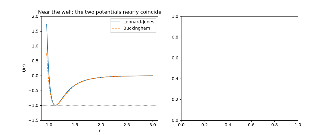
<matplotlib.legend.Legend object at 0x11b8efb60>

At short enough range, though, the Buckingham potential’s exponential repulsion is overtaken by its own unbounded dispersion attraction: past a spurious inner maximum, well inside the true minimum, it turns over and plunges toward -infinity rather than diverging to +infinity the way Lennard-Jones’s pure r**-12 repulsion does.

r_short = np.linspace(0.25, 0.9 * lj.r_min, 400)

axes[1].plot(r_short, lj.energy(r_short), label="Lennard-Jones")
axes[1].plot(r_short, buckingham.energy(r_short), label="Buckingham", linestyle="--")
axes[1].axhline(0.0, color="gray", linestyle=":", linewidth=0.8)
axes[1].set_xlabel("r")
axes[1].set_ylabel("U(r)")
axes[1].set_ylim(-20.0, 20.0)
axes[1].set_title("Short range: Buckingham's unphysical inner turnover")
axes[1].legend()

fig.tight_layout()
plt.show()