The Nose-Hoover thermostat: a friction variable that steers the temperature

Nose’s extended system, in Hoover’s friction-coefficient form, adds a single dynamical variable \(\xi\) to Newton’s equations:

\[\dot{\vec v}_i = \frac{\vec F_i}{m_i} - \xi \vec v_i, \qquad Q\dot\xi = \sum_i m_i v_i^2 - N_f k_B T_0 .\]

When the fluid is too hot, \(\xi\) grows positive and drains kinetic energy; when it is too cold, \(\xi\) turns negative and feeds energy back in. A Lennard-Jones fluid started well above the target temperature is run without a thermostat (NVE) and with NoseHooverThermostat at two thermostat masses \(Q\), recording the temperature and the friction coefficient \(\xi\).

import matplotlib.pyplot as plt

from chemistrykit.md.systems.lj_fluid import LJFluid
from chemistrykit.md.systems.thermostats import NoseHooverThermostat

T_target = 1.0
dt, n_steps = 0.004, 5000


def make_hot_fluid():
    fluid = LJFluid.from_lattice(n_per_side=6, density=0.6, temperature=T_target, cutoff=2.5, rng=0)
    fluid.velocities *= 1.8  # start well above the target temperature
    return fluid


fig, axes = plt.subplots(1, 2, figsize=(11, 4.5))
nve = make_hot_fluid()
result = nve.run(dt=dt, n_steps=n_steps, sample_every=10)
axes[0].plot(result.t, result.temperature, color="gray", label="NVE (no thermostat)")

for Q, color in [(5.0, "steelblue"), (50.0, "darkorange")]:
    fluid = make_hot_fluid()
    thermostat = NoseHooverThermostat(target_temperature=T_target, Q=Q)
    times, temps, xis = [], [], []
    for _ in range(n_steps // 10):
        fluid.run(dt=dt, n_steps=10, thermostat=thermostat, sample_every=10)
        times.append(fluid.t)
        temps.append(fluid.temperature())
        xis.append(thermostat.xi)
    axes[0].plot(times, temps, color=color, label=f"Nose-Hoover, Q = {Q:g}")
    axes[1].plot(times, xis, color=color, label=f"Q = {Q:g}")

axes[0].axhline(T_target, color="black", linestyle=":", linewidth=0.8, label="target T")
axes[0].set_xlabel("t")
axes[0].set_ylabel("instantaneous temperature")
axes[0].set_title("Temperature")
axes[0].legend(loc="upper right")
axes[1].axhline(0.0, color="black", linestyle=":", linewidth=0.8)
axes[1].set_xlabel("t")
axes[1].set_ylabel(r"friction coefficient $\xi$")
axes[1].set_title("The extended-system variable")
axes[1].legend()
fig.tight_layout()

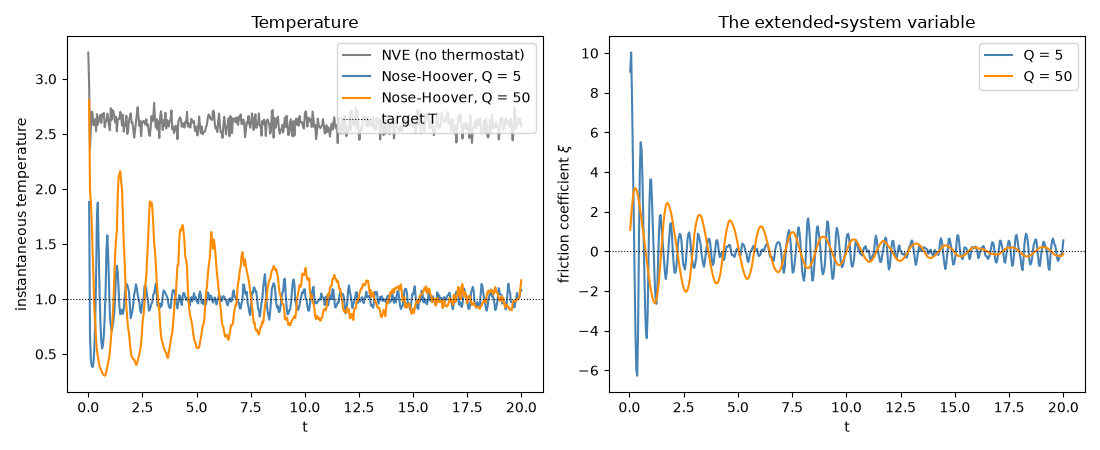
Without a thermostat the fluid stays hot. With Nose-Hoover the friction coefficient first rises to cool the fluid, overshoots, and then oscillates about zero, so the temperature swings back and forth around the target rather than being clamped to it; a heavier thermostat mass Q responds more slowly, with longer, gentler swings. Averaged over the second half of each run, the temperature sits close to the target:

for line in axes[0].get_lines()[1:3]:
    temps = line.get_ydata()
    print(f"{line.get_label()}: mean T over second half = {sum(temps[len(temps) // 2 :]) / (len(temps) - len(temps) // 2):.3f}")

plt.show()

Nose-Hoover, Q = 5: mean T over second half = 1.000
Nose-Hoover, Q = 50: mean T over second half = 0.999