Bussi-Donadio-Parrinello: stochastic velocity rescaling samples the canonical ensemble

Bussi, Donadio, and Parrinello (2007) kept Berendsen’s exponential relaxation of the kinetic energy \(K\) but added a stochastic term of exactly the right size,

\[dK = (\bar K - K)\frac{dt}{\tau} + 2\sqrt{\frac{K\bar K}{N_f\tau}}\,dW,\]

so that \(K\) samples its canonical distribution – a gamma distribution with mean \(\bar K = N_f k_B T_0/2\) and variance \(2\bar K^2/N_f\) – while \(\tau\) still sets how fast it gets there (StochasticVelocityRescalingThermostat). The same dense Lennard-Jones liquid is thermostatted with Berendsen coupling and with stochastic rescaling at the same \(\tau\), and the histogram of kinetic energies is compared with the canonical distribution.

import matplotlib.pyplot as plt
import numpy as np
from scipy.stats import gamma

from chemistrykit.md.systems.lj_fluid import LJFluid
from chemistrykit.md.systems.thermostats import BerendsenThermostat, StochasticVelocityRescalingThermostat

T0, tau, dt = 1.0, 0.1, 0.005
thermostats = {
    "Berendsen": BerendsenThermostat(T0, tau=tau),
    "stochastic velocity rescaling": StochasticVelocityRescalingThermostat(T0, tau=tau, rng=0),
}

fig, axes = plt.subplots(1, 2, figsize=(11, 4.5))
samples = {}
for (name, thermostat), color in zip(thermostats.items(), ["firebrick", "steelblue"]):
    liquid = LJFluid.from_lattice(n_per_side=5, density=0.8, temperature=2.0 * T0, cutoff=2.4, rng=1)
    result = liquid.run(dt=dt, n_steps=6000, thermostat=thermostat, sample_every=5)
    axes[0].plot(result.t, result.temperature, color=color, linewidth=0.8, label=name)
    samples[name] = result.kinetic_energy[result.t > 5.0]
    nf = liquid.degrees_of_freedom()

k_bar = 0.5 * nf * T0
axes[0].axhline(T0, color="black", linestyle=":", linewidth=0.8)
axes[0].set_xlabel("t")
axes[0].set_ylabel("instantaneous temperature")
axes[0].set_title(rf"Relaxation from $T=2$ (both $\tau$ = {tau})")
axes[0].legend()

K = np.linspace(0.7 * k_bar, 1.3 * k_bar, 300)
canonical = gamma(a=nf / 2, scale=T0)  # K is Gamma(N_f/2, k_B T_0)
for (name, ks), color in zip(samples.items(), ["firebrick", "steelblue"]):
    axes[1].hist(ks, bins=40, range=(K[0], K[-1]), density=True, alpha=0.5, color=color, label=name)
axes[1].plot(K, canonical.pdf(K), color="black", label="canonical (gamma)")
axes[1].set_xlabel("kinetic energy K")
axes[1].set_ylabel("probability density")
axes[1].set_title("Kinetic-energy distribution after equilibration")
axes[1].legend()
fig.tight_layout()

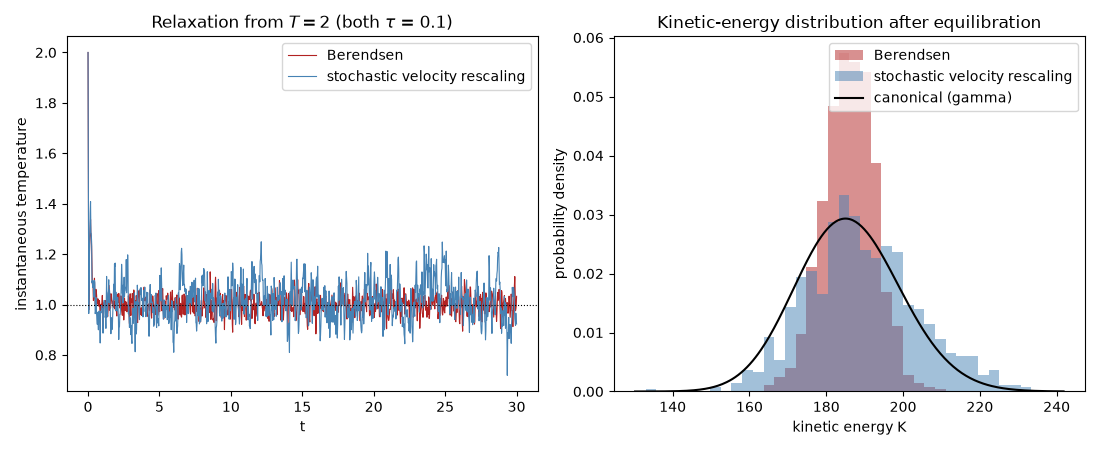
Both thermostats bring the liquid to the target temperature at the same rate, but only stochastic rescaling reproduces the canonical spread of the kinetic energy; Berendsen’s distribution is far too narrow:

print(f"canonical standard deviation of K: {canonical.std():.2f}")
for name, ks in samples.items():
    print(f"{name}: mean K = {ks.mean():.1f} (canonical {k_bar:.1f}), std = {ks.std():.2f}")

plt.show()

canonical standard deviation of K: 13.64
Berendsen: mean K = 186.0 (canonical 186.0), std = 6.70
stochastic velocity rescaling: mean K = 189.3 (canonical 186.0), std = 14.47