Visualizing a trajectory: XYZ files for VMD and OVITO

Molecular-dynamics results are usually inspected in a dedicated viewer such as VMD or OVITO, and the lowest common denominator they all read is the XYZ format: an atom count, a comment line, and one symbol x y z row per atom, repeated for every frame. write_xyz() writes a whole MDResult this way. It puts the periodic box in the extended-XYZ Lattice= comment that OVITO reads, and scales the Lennard-Jones reduced lengths to angstroms (\(\sigma = 3.405\) Å for argon), since viewers assume Å. 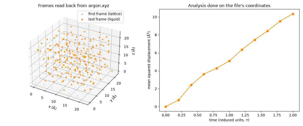The file is then read back with read_xyz() and a frame is drawn straight from it.

import os
import tempfile

import matplotlib.pyplot as plt
import numpy as np

from chemistrykit.md import LJFluid, read_xyz, write_xyz

SIGMA_ARGON = 3.405  # angstrom

fluid = LJFluid.from_lattice(n_per_side=6, density=0.8, temperature=1.2, rng=np.random.default_rng(1))
result = fluid.run(dt=0.005, n_steps=400, sample_every=40)

path = os.path.join(tempfile.mkdtemp(), "argon.xyz")
write_xyz(path, result, symbols="Ar", scale=SIGMA_ARGON, comment="liquid argon, LJ reduced units scaled to angstrom")

with open(path) as fh:
    head = [next(fh) for _ in range(4)]
print("".join(head))

traj = read_xyz(path, scale=SIGMA_ARGON)
print(f"{len(traj.comments)} frames of {len(traj.symbols)} atoms read back;", "max round-trip error:", float(np.abs(traj.positions - result.positions).max()))

216
Lattice="22.00755036 0 0 0 22.00755036 0 0 0 22.00755036" Properties=species:S:1:pos:R:3 Comment="liquid argon, LJ reduced units scaled to angstrom" Time=0
Ar 0.0000000000 0.0000000000 0.0000000000
Ar 0.0000000000 0.0000000000 3.6679250598

11 frames of 216 atoms read back; max round-trip error: 1.468336563448247e-11

fig = plt.figure(figsize=(12, 5))
ax = fig.add_subplot(1, 2, 1, projection="3d")
first, last = traj.positions[0] * SIGMA_ARGON, traj.positions[-1] * SIGMA_ARGON
ax.scatter(*first.T, s=12, color="steelblue", alpha=0.4, label="first frame (lattice)")
ax.scatter(*last.T, s=12, color="darkorange", label="last frame (liquid)")
ax.set_xlabel("x (Å)")
ax.set_ylabel("y (Å)")
ax.set_zlabel("z (Å)")
ax.set_title("Frames read back from argon.xyz")
ax.legend()

ax2 = fig.add_subplot(1, 2, 2)
L = result.box_length
disp = traj.positions - traj.positions[0]
disp -= L * np.round(disp / L)
ax2.plot(result.t, (disp**2).sum(axis=2).mean(axis=1) * SIGMA_ARGON**2, "o-", color="darkorange")
ax2.set_xlabel(r"time (reduced units, $\tau$)")
ax2.set_ylabel(r"mean squared displacement (Å$^2$)")
ax2.set_title("Analysis done on the file's coordinates")
fig.tight_layout()

plt.show()