Debye light scattering measures Mw; osmometry measures Mn

Debye (1944) showed that the light scattered by a dilute polymer solution, extrapolated to zero angle and zero concentration, gives an absolute molar mass – the weight average, because each chain scatters in proportion to the square of its mass (rayleigh_ratio_dilute_mixture()). Osmotic pressure counts molecules instead and gives the number average (osmotic_pressure_dilute_mixture()). Here a blend of two narrow fractions is “measured” both ways, and a Debye plot \(Kc/R_0=1/M_w+2A_2c\) (debye_Kc_over_R()) is extrapolated to \(c=0\).

import matplotlib.pyplot as plt
import numpy as np

from chemistrykit.polymer.systems.light_scattering import (
    debye_Kc_over_R,
    osmotic_pressure_dilute_mixture,
    rayleigh_ratio_dilute_mixture,
)
from chemistrykit.polymer.systems.molecular_weight_distribution import (
    number_average_molar_mass,
    polydispersity_index,
    weight_average_molar_mass,
)

# Equal masses of a 20 kg/mol and a 500 kg/mol fraction.
M_i = np.array([20.0, 500.0])  # kg/mol
w_i = np.array([0.5, 0.5])  # mass fractions
Mn = number_average_molar_mass(w_i / M_i, M_i)
Mw = weight_average_molar_mass(w_i / M_i, M_i)
print(f"True Mn = {Mn:.1f} kg/mol, Mw = {Mw:.1f} kg/mol, PDI = {polydispersity_index(Mn, Mw):.2f}")

True Mn = 38.5 kg/mol, Mw = 260.0 kg/mol, PDI = 6.76

“Measure” each at a dilute total concentration c (kg/m^3).

c_total = 1.0
K, T = 1.0, 298.15
R0 = rayleigh_ratio_dilute_mixture(c_total * w_i, M_i, K)
Pi = osmotic_pressure_dilute_mixture(c_total * w_i, M_i, T)
M_light = R0 / (K * c_total)
M_osmo = 8.314462618 * T * c_total / Pi
print(f"Light scattering apparent M = {M_light:.1f} kg/mol  (= Mw)")
print(f"Osmometry apparent M        = {M_osmo:.1f} kg/mol  (= Mn)")

Light scattering apparent M = 260.0 kg/mol  (= Mw)
Osmometry apparent M        = 38.5 kg/mol  (= Mn)

Debye plot with a second virial coefficient; the intercept is 1/Mw.

A2 = 2.0e-4
c = np.linspace(0.5, 5.0, 8)
rng = np.random.default_rng(1)
y = debye_Kc_over_R(c, Mw, A2) * (1 + 0.005 * rng.standard_normal(c.size))
slope, intercept = np.polyfit(c, y, 1)
print(f"Debye-plot intercept -> Mw = {1 / intercept:.1f} kg/mol; slope -> A2 = {slope / 2:.2e}")

fig, axes = plt.subplots(1, 2, figsize=(11, 4.2))
cc = np.linspace(0, 5.0, 50)
axes[0].plot(c, y, "o", label="simulated data")
axes[0].plot(cc, intercept + slope * cc, "k-", lw=0.8, label="linear extrapolation")
axes[0].axhline(1 / Mn, color="crimson", ls="--", label="1/Mn (would be wrong)")
axes[0].set_xlabel("c (kg/m$^3$)")
axes[0].set_ylabel(r"$Kc/R_0$ (mol/kg)")
axes[0].set_title("Debye plot: intercept = 1/Mw")
axes[0].legend()

axes[1].bar(["Mn (osmometry)", "Mw (light scattering)"], [M_osmo, M_light], color=["crimson", "steelblue"])
axes[1].set_ylabel("apparent M (kg/mol)")
axes[1].set_title("Same blend, two different averages")
plt.tight_layout()
plt.show()

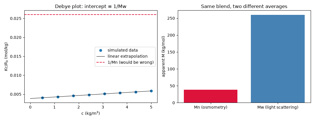
Debye-plot intercept -> Mw = 259.6 kg/mol; slope -> A2 = 2.00e-04