Flory-Huggins lattice theory: free energy of mixing and the phase diagram

Flory and Huggins (1941-1942) placed polymer segments and solvent on a lattice to get the mixing free energy per site (flory_huggins_free_energy())

\[\frac{\Delta F_\text{mix}}{k_BT} = \frac{\phi}{N}\ln\phi + (1-\phi)\ln(1-\phi) + \chi\phi(1-\phi)\]

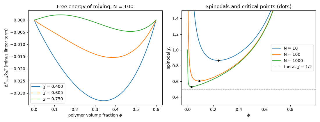
Below the critical \(\chi_c\) the curve is convex and the solution is stable; above it a concave region appears and the solution phase separates. The spinodal (flory_huggins_spinodal_chi()) has its minimum at the critical point (flory_huggins_critical_point()), which moves to \(\phi_c\to0\), \(\chi_c\to1/2\) (the theta point) as the chains get longer.

import matplotlib.pyplot as plt
import numpy as np

from chemistrykit.polymer.systems.flory_huggins import (
    flory_huggins_critical_point,
    flory_huggins_free_energy,
    flory_huggins_spinodal_chi,
)

N = 100
phi_c, chi_c = flory_huggins_critical_point(N)
print(f"N = {N}: phi_c = {phi_c:.4f}, chi_c = {chi_c:.4f}")
for Nv in (1, 10, 100, 1000, 10**6):
    pc, cc = flory_huggins_critical_point(Nv)
    print(f"  N = {Nv:>7}: phi_c = {pc:.4f}, chi_c = {cc:.4f}")

N = 100: phi_c = 0.0909, chi_c = 0.6050
  N =       1: phi_c = 0.5000, chi_c = 2.0000
  N =      10: phi_c = 0.2403, chi_c = 0.8662
  N =     100: phi_c = 0.0909, chi_c = 0.6050
  N =    1000: phi_c = 0.0307, chi_c = 0.5321
  N = 1000000: phi_c = 0.0010, chi_c = 0.5010

phi = np.linspace(1e-4, 0.6, 600)
fig, axes = plt.subplots(1, 2, figsize=(11, 4.2))
for chi in (0.4, chi_c, 0.75):
    F = flory_huggins_free_energy(phi, N, chi)
    # subtract the straight chord from phi=0 to phi=0.6 so the curvature is visible
    axes[0].plot(phi, F - F[-1] * phi / phi[-1], label=rf"$\chi$ = {chi:.3f}")
axes[0].set_xlabel(r"polymer volume fraction $\phi$")
axes[0].set_ylabel(r"$\Delta F_{mix}/k_BT$ (minus linear term)")
axes[0].set_title(f"Free energy of mixing, N = {N}")
axes[0].legend()

phi_s = np.linspace(1e-3, 0.95, 800)
for Nv in (10, 100, 1000):
    axes[1].plot(phi_s, flory_huggins_spinodal_chi(phi_s, Nv), label=f"N = {Nv}")
    axes[1].plot(*flory_huggins_critical_point(Nv), "ko", ms=4)
axes[1].axhline(0.5, color="gray", ls="--", lw=0.8, label=r"theta, $\chi$ = 1/2")
axes[1].set_ylim(0.3, 1.5)
axes[1].set_xlabel(r"$\phi$")
axes[1].set_ylabel(r"spinodal $\chi_s$")
axes[1].set_title("Spinodals and critical points (dots)")
axes[1].legend()
plt.tight_layout()
plt.show()