The Debye-Huckel limiting law: log gamma is linear in the square root of I

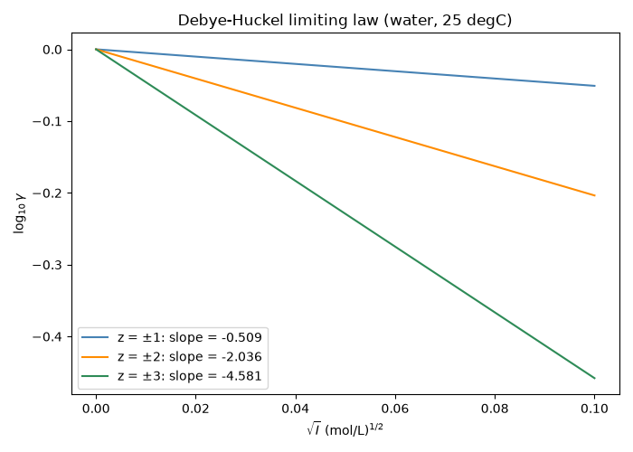
Debye and Huckel’s screening theory predicts that at low ionic strength

\[\log_{10}\gamma = -A z^2 \sqrt{I},\]

a straight line in \(\sqrt{I}\) whose slope scales with the square of the ion’s charge (activity_coefficient_debye_huckel_limiting()). The ionic strength \(I = \frac{1}{2}\sum_i c_i z_i^2\) that controls the screening is computed with ionic_strength().

import matplotlib.pyplot as plt
import numpy as np

from chemistrykit.solutions.systems.activity import (
    DEBYE_HUCKEL_A_25C,
    activity_coefficient_debye_huckel_limiting,
    ionic_strength,
)

sqrt_I = np.linspace(0.0, 0.1, 50)  # I up to 0.01 M, the limiting-law regime

fig, ax = plt.subplots(figsize=(7, 5))
for z, color in [(1, "steelblue"), (2, "darkorange"), (3, "seagreen")]:
    log_gamma = [np.log10(activity_coefficient_debye_huckel_limiting(z, s**2)) for s in sqrt_I]
    ax.plot(sqrt_I, log_gamma, color=color, label=f"z = ±{z}: slope = {-DEBYE_HUCKEL_A_25C * z**2:.3f}")
ax.set_xlabel(r"$\sqrt{I}$ (mol/L)$^{1/2}$")
ax.set_ylabel(r"$\log_{10}\gamma$")
ax.set_title("Debye-Huckel limiting law (water, 25 degC)")
ax.legend()
fig.tight_layout()

Ionic strength of some dilute solutions, and the resulting activity coefficients of their ions:

solutions = {
    "0.001 M NaCl": ([0.001, 0.001], [1, -1]),
    "0.001 M CaCl2": ([0.001, 0.002], [2, -1]),
    "0.001 M MgSO4": ([0.001, 0.001], [2, -2]),
}
for name, (c, z) in solutions.items():
    I = ionic_strength(c, z)
    gammas = ", ".join(f"z={zi:+d}: {activity_coefficient_debye_huckel_limiting(zi, I):.3f}" for zi in z)
    print(f"{name:14s}: I = {I:.4f} M; gamma({gammas})")

plt.show()

0.001 M NaCl  : I = 0.0010 M; gamma(z=+1: 0.964, z=-1: 0.964)
0.001 M CaCl2 : I = 0.0030 M; gamma(z=+2: 0.774, z=-1: 0.938)
0.001 M MgSO4 : I = 0.0040 M; gamma(z=+2: 0.743, z=-2: 0.743)