Jannik Bjerrum’s stepwise metal-ammine formation

Copper(II) binds ammonia one ligand at a time, \(Cu(NH_3)_{n-1}^{2+} + NH_3 \rightleftharpoons Cu(NH_3)_n^{2+}\), with stepwise constants \(K_1 > K_2 > K_3 > K_4\). Bjerrum showed that the whole ladder follows from the free-ligand concentration alone. The fractions \(\alpha_n\) (complex_fractions()) and the mean number of bound ligands \(\bar n\) (average_ligand_number(), Bjerrum’s formation function) are functions of \(p[NH_3]\) only. His “half-\(\bar n\)” rule runs the logic backwards: where \(\bar n = n - \tfrac12\), \(p[NH_3] \approx \log K_n\), so the constants can be read off a measured formation curve. The stepwise constants below are of the size Bjerrum measured for Cu(II)-ammonia.

import matplotlib.pyplot as plt
import numpy as np

from chemistrykit.solutions import average_ligand_number, complex_fractions, cumulative_formation_constants, solve_complexation

log_K = np.array([4.31, 3.67, 3.04, 2.30])
beta = cumulative_formation_constants(10.0**log_K)

pL = np.linspace(0.0, 6.0, 600)
L = 10.0**-pL
alpha = complex_fractions(L, beta)
nbar = average_ligand_number(L, beta)

fig, axes = plt.subplots(1, 2, figsize=(12, 4.8))
for n, a in enumerate(alpha):
    axes[0].plot(pL, a, label=rf"Cu(NH$_3$)$_{n}^{{2+}}$")
axes[0].invert_xaxis()
axes[0].set_xlabel(r"p[NH$_3$] = $-\log$[NH$_3$]")
axes[0].set_ylabel(r"fraction of copper, $\alpha_n$")
axes[0].set_title("Species distribution")
axes[0].legend()

axes[1].plot(pL, nbar, color="black")
estimates = []
for n in range(1, 5):
    p_half = float(np.interp(-(n - 0.5), -nbar, pL))  # nbar decreases with pL
    estimates.append(p_half)
    axes[1].plot(p_half, n - 0.5, "o", color="darkorange")
axes[1].invert_xaxis()
axes[1].set_xlabel(r"p[NH$_3$]")
axes[1].set_ylabel(r"formation function $\bar n$")
axes[1].set_title(r"Half-$\bar n$ estimates of $\log K_n$ (dots)")
fig.tight_layout()

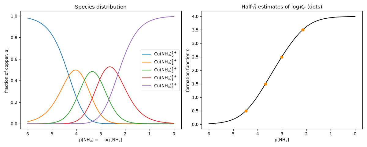
The half-\(\bar n\) estimates land close to the true constants; the small offsets come from overlap between neighboring steps.

for n, (true, est) in enumerate(zip(log_K, estimates, strict=True), start=1):
    print(f"log K{n}: true {true:.2f}, half-nbar estimate {est:.2f}")

log K1: true 4.31, half-nbar estimate 4.48
log K2: true 3.67, half-nbar estimate 3.68
log K3: true 3.04, half-nbar estimate 3.01
log K4: true 2.30, half-nbar estimate 2.15

Given only the totals, solve_complexation() solves the ligand mass balance for the free ammonia concentration:

eq = solve_complexation(M_total=0.01, L_total=0.05, beta=beta)
print(f"free NH3 = {eq.free_ligand:.2e} M, nbar = {eq.average_ligand_number:.2f}")
print("species (M):", np.array2string(eq.species, precision=2))

plt.show()

free NH3 = 1.31e-02 M, nbar = 3.69
species (M): [1.15e-08 3.08e-06 1.89e-04 2.71e-03 7.09e-03]