The Maxwell-Boltzmann speed distribution

MaxwellBoltzmannSpeedDistribution at two temperatures, with the most-probable, mean, and rms speeds marked – their ratios are a fixed, temperature-independent property of the distribution’s shape.

import matplotlib.pyplot as plt
import numpy as np

from chemistrykit.statmech import MaxwellBoltzmannSpeedDistribution

mass = 6.63e-26  # argon-like, kg

fig, ax = plt.subplots(figsize=(7, 5))
for T, color in [(200.0, "steelblue"), (800.0, "crimson")]:
    dist = MaxwellBoltzmannSpeedDistribution(mass=mass, temperature=T)
    v = np.linspace(0.0, 2500.0, 400)
    ax.plot(v, dist.pdf(v), color=color, label=f"T = {T:.0f} K")
    ax.axvline(dist.most_probable_speed(), color=color, linestyle=":", linewidth=0.8)

ax.set_xlabel("speed (m/s)")
ax.set_ylabel("probability density")
ax.set_title("Maxwell-Boltzmann speed distribution at two temperatures")
ax.legend()
fig.tight_layout()

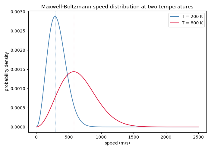
The three characteristic speeds stand in a fixed ratio, independent of temperature or mass – a purely geometric property of the distribution’s shape:

dist = MaxwellBoltzmannSpeedDistribution(mass=mass, temperature=298.15)
vp, vbar, vrms = dist.most_probable_speed(), dist.mean_speed(), dist.rms_speed()
print(f"v_p : v_bar : v_rms = 1 : {vbar / vp:.4f} : {vrms / vp:.4f}")
print(f"expected             = 1 : {np.sqrt(8.0 / np.pi) / np.sqrt(2.0):.4f} : {np.sqrt(3.0) / np.sqrt(2.0):.4f}")

plt.show()

v_p : v_bar : v_rms = 1 : 1.1284 : 1.2247
expected             = 1 : 1.1284 : 1.2247