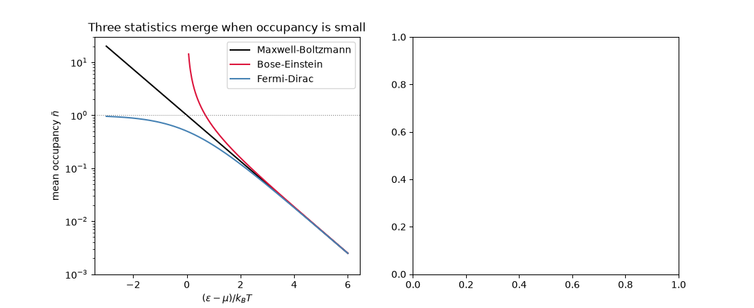
Bose-Einstein and Fermi-Dirac statistics reduce to Maxwell-Boltzmann

Bose and Einstein (1924-25) and Fermi and Dirac (1926) found the mean occupancy of a single-particle state of energy \(\varepsilon\) for indistinguishable bosons and fermions:

\[\bar n_{\text{BE}}=\frac{1}{e^{(\varepsilon-\mu)/k_BT}-1},\qquad \bar n_{\text{FD}}=\frac{1}{e^{(\varepsilon-\mu)/k_BT}+1},\qquad \bar n_{\text{MB}}=e^{-(\varepsilon-\mu)/k_BT}\]

When \((\varepsilon-\mu)/k_BT\gg1\), i.e. every state is sparsely occupied, both quantum distributions collapse onto the classical Maxwell-Boltzmann one. For an ideal gas the fugacity is \(z=e^{\mu/k_BT}\approx n\Lambda^3\), so the “degeneracy parameter” \(n\Lambda^3\), computed with thermal_de_broglie_wavelength(), says how close to the quantum regime a real gas is. (These occupancies are written out with NumPy here; the package’s partition functions use the classical limit throughout.)

import matplotlib.pyplot as plt
import numpy as np
import scipy.constants as sc

from chemistrykit.constants import K_B
from chemistrykit.statmech import thermal_de_broglie_wavelength

x = np.linspace(-3.0, 6.0, 400)  # (epsilon - mu) / k_B T
n_mb = np.exp(-x)
n_fd = 1.0 / (np.exp(x) + 1.0)
x_be = x[x > 0.05]
n_be = 1.0 / np.expm1(x_be)

fig, axes = plt.subplots(1, 2, figsize=(11, 4.5))
axes[0].semilogy(x, n_mb, color="black", label="Maxwell-Boltzmann")
axes[0].semilogy(x_be, n_be, color="crimson", label="Bose-Einstein")
axes[0].semilogy(x, n_fd, color="steelblue", label="Fermi-Dirac")
axes[0].axhline(1.0, color="gray", linestyle=":", linewidth=0.8)
axes[0].set_ylim(1e-3, 30.0)
axes[0].set_xlabel(r"$(\varepsilon - \mu) / k_BT$")
axes[0].set_ylabel(r"mean occupancy $\bar n$")
axes[0].set_title("Three statistics merge when occupancy is small")
axes[0].legend()

<matplotlib.legend.Legend object at 0x11c0e7380>

Degeneracy parameter n Lambda^3 for real gases at 1 bar: whenever it is tiny, every state has occupancy ~ n Lambda^3 << 1 and the classical limit (right half of the left panel) applies.

T = np.logspace(0.0, 3.0, 300)
n = 1.0e5 / (K_B * T)
gases = [("He", 4.0026, "crimson"), ("H2", 2.016, "darkorange"), ("Ar", 39.948, "steelblue")]
for name, mass_u, color in gases:
    axes[1].loglog(T, n * thermal_de_broglie_wavelength(mass_u * sc.atomic_mass, T) ** 3, color=color, label=name)
axes[1].axhline(1.0, color="gray", linestyle="--", label=r"$n\Lambda^3 = 1$ (quantum regime)")
axes[1].set_xlabel("T (K)")
axes[1].set_ylabel(r"$n\Lambda^3$ at 1 bar")
axes[1].set_title("How far real gases are from quantum degeneracy")
axes[1].legend()
fig.tight_layout()

for x_check in (1.0, 3.0, 6.0):
    rel_be = (1.0 / np.expm1(x_check) - np.exp(-x_check)) / np.exp(-x_check)
    rel_fd = (1.0 / (np.exp(x_check) + 1.0) - np.exp(-x_check)) / np.exp(-x_check)
    print(f"(eps-mu)/kT = {x_check}: BE differs from MB by {rel_be:+.2%}, FD by {rel_fd:+.2%}")

plt.show()

(eps-mu)/kT = 1.0: BE differs from MB by +58.20%, FD by -26.89%
(eps-mu)/kT = 3.0: BE differs from MB by +5.24%, FD by -4.74%
(eps-mu)/kT = 6.0: BE differs from MB by +0.25%, FD by -0.25%