Debye’s T-cubed law for the heat capacity of a solid

Debye (1912) replaced Einstein’s single vibrational frequency with the full spectrum of lattice sound waves, \(g(\nu)\propto\nu^2\) up to a cutoff \(\nu_D\). DebyeSolid gives

\[C_V=9R\left(\frac{T}{\Theta_D}\right)^3\int_0^{\Theta_D/T} \frac{x^4e^x}{(e^x-1)^2}\,dx \;\xrightarrow{T\to0}\;\frac{12\pi^4}{5}R\left(\frac{T}{\Theta_D}\right)^3\]

per mole of atoms. The low-frequency acoustic modes stay thermally active at low temperature, so \(C_V\) falls as \(T^3\). An Einstein solid with a comparable frequency falls exponentially, much faster than measured low-temperature heat capacities do.

import matplotlib.pyplot as plt
import numpy as np

from chemistrykit.constants import K_B, H, R
from chemistrykit.statmech import DebyeSolid, VibrationalPartitionFunctionHarmonic

theta_D = 343.0  # copper, K (Kittel, Introduction to Solid State Physics, Table 5.1)
copper = DebyeSolid(debye_temperature=theta_D)

# The Einstein temperature that best matches Debye at high T is Theta_E = sqrt(3/5) Theta_D.
einstein_mode = VibrationalPartitionFunctionHarmonic(frequency=np.sqrt(3.0 / 5.0) * theta_D * K_B / H)

T = np.linspace(1.0, 600.0, 400)
Cv_debye = copper.heat_capacity_v(T)
Cv_einstein = 3.0 * einstein_mode.heat_capacity_v(T)

fig, axes = plt.subplots(1, 2, figsize=(11, 4.5))
axes[0].plot(T / theta_D, Cv_debye / (3 * R), color="steelblue", label="Debye")
axes[0].plot(T / theta_D, Cv_einstein / (3 * R), color="crimson", linestyle="--", label="Einstein")
axes[0].axhline(1.0, color="gray", linestyle=":", linewidth=0.8, label="Dulong-Petit 3R")
axes[0].set_xlabel(r"$T / \Theta_D$")
axes[0].set_ylabel(r"$C_V / 3R$")
axes[0].set_title("Debye vs. Einstein solid")
axes[0].legend()

T_low = np.logspace(-0.5, 2.0, 200)
axes[1].loglog(T_low, copper.heat_capacity_v(T_low), color="steelblue", label="Debye")
axes[1].loglog(T_low, copper.low_temperature_heat_capacity(T_low), color="black", linestyle=":", label=r"$T^3$ law")
axes[1].loglog(T_low, 3.0 * einstein_mode.heat_capacity_v(T_low), color="crimson", linestyle="--", label="Einstein")
axes[1].set_ylim(1e-6, 30.0)
axes[1].set_xlabel("T (K)")
axes[1].set_ylabel(r"$C_V$ (J mol$^{-1}$ K$^{-1}$)")
axes[1].set_title(r"Copper ($\Theta_D$ = 343 K): the $T^3$ law")
axes[1].legend()
fig.tight_layout()

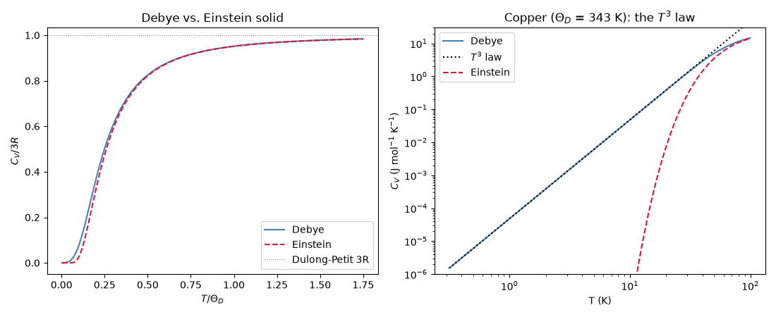
Below about Theta_D / 50 the full Debye result and the T^3 law agree to better than 0.1 %:

for t in (2.0, 5.0, 20.0, 100.0):
    ratio = copper.heat_capacity_v(t) / copper.low_temperature_heat_capacity(t)
    print(f"T = {t:5.1f} K: Cv = {copper.heat_capacity_v(t):.4e} J/(mol K), Cv / T^3-law = {ratio:.4f}")

plt.show()

T =   2.0 K: Cv = 3.8535e-04 J/(mol K), Cv / T^3-law = 1.0000
T =   5.0 K: Cv = 6.0211e-03 J/(mol K), Cv / T^3-law = 1.0000
T =  20.0 K: Cv = 3.8529e-01 J/(mol K), Cv / T^3-law = 0.9998
T = 100.0 K: Cv = 1.4766e+01 J/(mol K), Cv / T^3-law = 0.3066