Mayer’s cluster expansion: the second virial coefficient

Mayer (1937) expanded a real gas’s partition function in clusters of the Mayer function \(f(r)=e^{-u(r)/k_BT}-1\). The first correction to the ideal-gas law, \(PV_m/RT=1+B_2(T)/V_m+\cdots\), is

\[B_2(T)=-2\pi N_A\int_0^\infty\left(e^{-u(r)/k_BT}-1\right)r^2\,dr .\]

second_virial_coefficient() evaluates this integral for any pair potential. Below it is applied to hard spheres (\(B_2=\frac{2\pi}{3}N_A\sigma^3\), independent of temperature) and to an argon-like Lennard-Jones potential, whose \(B_2\) changes sign at the Boyle temperature, \(T_B\approx3.42\,\epsilon/k_B\).

import matplotlib.pyplot as plt
import numpy as np
from scipy.optimize import brentq

from chemistrykit.constants import K_B, NA
from chemistrykit.md.systems.lj_fluid import LennardJones
from chemistrykit.statmech import second_virial_coefficient

# Argon-like Lennard-Jones parameters (Hirschfelder, Curtiss & Bird)
epsilon, sigma = 119.8 * K_B, 3.405e-10
lj = LennardJones(epsilon=epsilon, sigma=sigma)
hard_sphere = lambda r: np.inf if r < sigma else 0.0
B_hs = 2.0 * np.pi / 3.0 * NA * sigma**3

T = np.linspace(60.0, 1500.0, 150)
B_lj = np.array([second_virial_coefficient(lj.energy, t, sigma) for t in T])
T_boyle = brentq(lambda t: second_virial_coefficient(lj.energy, t, sigma), 200.0, 1000.0)

fig, axes = plt.subplots(1, 2, figsize=(11, 4.5))
r = np.linspace(0.85, 3.0, 400) * sigma
for t, color in [(100.0, "crimson"), (400.0, "darkorange"), (1500.0, "steelblue")]:
    axes[0].plot(r / sigma, np.expm1(-lj.energy(r) / (K_B * t)), color=color, label=f"T = {t:.0f} K")
axes[0].axhline(0.0, color="gray", linewidth=0.8)
axes[0].set_ylim(-1.2, 2.5)
axes[0].set_xlabel(r"$r / \sigma$")
axes[0].set_ylabel(r"Mayer function $f(r) = e^{-u/k_BT} - 1$")
axes[0].set_title("The integrand: repulsion (f < 0) vs. attraction (f > 0)")
axes[0].legend()

axes[1].plot(T, B_lj * 1e6, color="steelblue", label="Lennard-Jones")
axes[1].axhline(B_hs * 1e6, color="gray", linestyle="--", label="hard spheres")
axes[1].axhline(0.0, color="black", linewidth=0.6)
axes[1].axvline(T_boyle, color="crimson", linestyle=":", label=f"Boyle temperature {T_boyle:.0f} K")
axes[1].set_xlabel("T (K)")
axes[1].set_ylabel(r"$B_2$ (cm$^3$ mol$^{-1}$)")
axes[1].set_title("Second virial coefficient of an argon-like gas")
axes[1].legend()
fig.tight_layout()

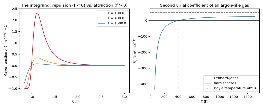
Consequences for the gas: at 1 bar the compressibility factor is Z = PV/RT ~ 1 + B_2 P / RT. Attraction makes Z < 1 below the Boyle temperature; repulsion makes Z > 1 above it.

print(f"hard-sphere B_2 = {B_hs * 1e6:.2f} cm^3/mol")
print(f"Boyle temperature = {T_boyle:.1f} K = {T_boyle / (epsilon / K_B):.4f} epsilon/k_B")
for t in (150.0, 300.0, 600.0):
    B2 = second_virial_coefficient(lj.energy, t, sigma)
    print(f"T = {t:.0f} K: B_2 = {B2 * 1e6:7.2f} cm^3/mol, Z(1 bar) = {1 + B2 * 1.0e5 / (8.314462618 * t):.5f}")

plt.show()

hard-sphere B_2 = 49.79 cm^3/mol
Boyle temperature = 409.5 K = 3.4179 epsilon/k_B
T = 150 K: B_2 =  -84.57 cm^3/mol, Z(1 bar) = 0.99322
T = 300 K: B_2 =  -15.46 cm^3/mol, Z(1 bar) = 0.99938
T = 600 K: B_2 =   12.16 cm^3/mol, Z(1 bar) = 1.00024