Polanyi’s potential theory and the Dubinin-Radushkevich characteristic curve

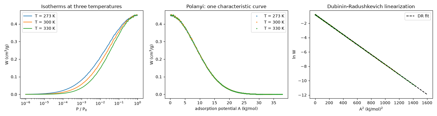
Polanyi (1914) described adsorption by the potential \(A = RT\ln(P_0/P)\) (polanyi_potential()) and claimed that the filled pore volume depends on \(A\) alone, through one characteristic curve that does not change with temperature. Dubinin and Radushkevich (1947) gave that curve for microporous carbons as \(W = W_0\exp[-(A/E)^2]\) (dubinin_radushkevich_loading()). Below, isotherms measured at three temperatures look different against \(P/P_0\) but fall onto a single curve when replotted against \(A\). A Dubinin-Radushkevich fit then recovers the pore volume \(W_0\) and the characteristic energy \(E\) (fit_dubinin_radushkevich()).

import matplotlib.pyplot as plt
import numpy as np

from chemistrykit.constants import R
from chemistrykit.surface.systems.dubinin import DubininRadushkevichIsotherm, fit_dubinin_radushkevich, polanyi_potential

W0, E = 0.45, 12.0e3  # cm^3/g, J/mol
dH_vap, T_ref, P0_ref = 30.0e3, 300.0, 10.0e3  # simple Clausius-Clapeyron vapor pressure, Pa


def P0_of(T):
    return P0_ref * np.exp(-dH_vap / R * (1.0 / T - 1.0 / T_ref))


temperatures = [273.0, 300.0, 330.0]
x = np.logspace(-6, -0.01, 200)  # P/P0
rng = np.random.default_rng(11)
data = {}
for T in temperatures:
    iso = DubininRadushkevichIsotherm(W0=W0, E=E, P0=P0_of(T), T=T)
    P = x * iso.P0
    W = iso.loading(P) * (1.0 + rng.normal(scale=0.005, size=P.shape))
    data[T] = (P, W, polanyi_potential(P, iso.P0, T))

P, W, _ = data[300.0]
mask = (P / P0_of(300.0)) < 0.2
fit = fit_dubinin_radushkevich(P[mask], W[mask], P0=P0_of(300.0), T=300.0)
print(f"True   (W0, E) = ({W0}, {E / 1e3:.1f} kJ/mol)")
print(f"Fitted (W0, E) = ({fit.W0:.4f}, {fit.E / 1e3:.2f} kJ/mol), R^2 = {fit.r_squared:.5f}")

True   (W0, E) = (0.45, 12.0 kJ/mol)
Fitted (W0, E) = (0.4502, 12.00 kJ/mol), R^2 = 1.00000

fig, axes = plt.subplots(1, 3, figsize=(15, 4))
for T, (P, W, A) in data.items():
    axes[0].semilogx(P / P0_of(T), W, label=f"T = {T:.0f} K")
    axes[1].plot(A / 1e3, W, ".", markersize=3, label=f"T = {T:.0f} K")
    axes[2].plot((A / 1e3) ** 2, np.log(W), ".", markersize=3)
axes[0].set_xlabel("P / P$_0$")
axes[0].set_ylabel("W (cm$^3$/g)")
axes[0].set_title("Isotherms at three temperatures")
axes[0].legend()
axes[1].set_xlabel("adsorption potential A (kJ/mol)")
axes[1].set_ylabel("W (cm$^3$/g)")
axes[1].set_title("Polanyi: one characteristic curve")
axes[1].legend()
A2 = np.linspace(0, 1600, 50)
axes[2].plot(A2, np.log(fit.W0) - A2 / (fit.E / 1e3) ** 2, "k--", label="DR fit")
axes[2].set_xlabel("A$^2$ (kJ/mol)$^2$")
axes[2].set_ylabel("ln W")
axes[2].set_title("Dubinin-Radushkevich linearization")
axes[2].legend()
plt.tight_layout()
plt.show()