The Freundlich adsorption isotherm

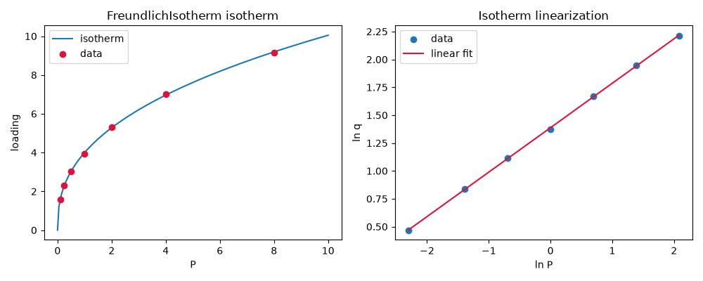
FreundlichIsotherm models the empirical power law \(q=K_fP^{1/n}\), useful for a heterogeneous surface where Langmuir’s single-site-energy assumption breaks down. Unlike Langmuir, it has no saturation limit, so extrapolating it far beyond the fitted pressure range is unphysical. fit_freundlich() recovers (Kf, n) via the standard log q vs. log P linearization.

import matplotlib.pyplot as plt
import numpy as np

from chemistrykit.surface.systems.freundlich import FreundlichIsotherm, fit_freundlich
from chemistrykit.surface.visualizers.surface_plots import plot_isotherm, plot_linearization

Kf_true, n_true = 4.0, 2.5
iso = FreundlichIsotherm(Kf=Kf_true, n=n_true)

print(f"Loading at P=1 (should equal Kf exactly): {iso.loading(1.0):.6f}")

Loading at P=1 (should equal Kf exactly): 4.000000

rng = np.random.default_rng(1)
P_data = np.array([0.1, 0.25, 0.5, 1.0, 2.0, 4.0, 8.0])
q_data = iso.loading(P_data) * (1.0 + rng.normal(scale=0.01, size=P_data.shape))

fit = fit_freundlich(P_data, q_data)
print(f"\nTrue (Kf, n)   = ({Kf_true}, {n_true})")
print(f"Fitted (Kf, n) = ({fit.Kf:.4f}, {fit.n:.4f})")
print(f"R^2 of linearized fit: {fit.r_squared:.6f}")

True (Kf, n)   = (4.0, 2.5)
Fitted (Kf, n) = (4.0055, 2.5087)
R^2 of linearized fit: 0.999847

fig, axes = plt.subplots(1, 2, figsize=(10, 4))
plot_isotherm(iso, P_max=10.0, P_data=P_data, q_data=q_data, ax=axes[0])

x_lin = np.log(P_data)
y_lin = np.log(q_data)
plot_linearization(x_lin, y_lin, fit=(1.0 / fit.n, np.log(fit.Kf)), ax=axes[1], xlabel="ln P", ylabel="ln q")
plt.tight_layout()
plt.show()