The Gibbs adsorption equation: surface excess from surface tension

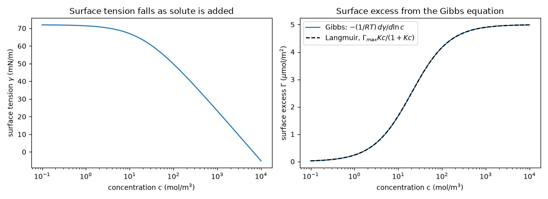
Gibbs showed that the amount of a dilute solute held at a liquid surface, the surface excess \(\Gamma\), follows from how the surface tension changes with concentration: \(\Gamma = -(1/RT)\,d\gamma/d\ln c\). So a surfactant that lowers \(\gamma\) must be concentrated at the surface, and no one has to look at the surface itself. This example takes Szyszkowski-type surface-tension data (szyszkowski_surface_tension()) for an aqueous fatty-acid-like solute and applies gibbs_surface_excess(). It recovers a saturating Langmuir curve for \(\Gamma\) and, from the plateau, the area each adsorbed molecule occupies.

import matplotlib.pyplot as plt
import numpy as np

from chemistrykit.constants import NA
from chemistrykit.surface.systems.gibbs_adsorption import gibbs_surface_excess, szyszkowski_surface_tension
from chemistrykit.surface.systems.langmuir import langmuir_coverage

T = 298.15
gamma0, Gamma_max, K = 0.0720, 5.0e-6, 0.05  # N/m, mol/m^2, m^3/mol
c = np.logspace(-1, 4, 800)  # mol/m^3
gamma = szyszkowski_surface_tension(c, gamma0, Gamma_max, K, T)

Gamma = gibbs_surface_excess(c, gamma, T)
expected = Gamma_max * langmuir_coverage(K, c)
print(f"Max relative deviation from Langmuir: {np.max(np.abs(Gamma[1:-1] / expected[1:-1] - 1)):.2e}")
area = 1.0 / (Gamma[-2] * NA) * 1e20
print(f"Area per molecule at the plateau: {area:.1f} A^2")

Max relative deviation from Langmuir: 3.41e-05
Area per molecule at the plateau: 33.3 A^2

fig, axes = plt.subplots(1, 2, figsize=(11, 4))
axes[0].semilogx(c, gamma * 1e3)
axes[0].set_xlabel("concentration c (mol/m$^3$)")
axes[0].set_ylabel(r"surface tension $\gamma$ (mN/m)")
axes[0].set_title("Surface tension falls as solute is added")

axes[1].semilogx(c, Gamma * 1e6, label="Gibbs: $-(1/RT)\\,d\\gamma/d\\ln c$")
axes[1].semilogx(c, expected * 1e6, "k--", label="Langmuir, $\\Gamma_{max}Kc/(1+Kc)$")
axes[1].set_xlabel("concentration c (mol/m$^3$)")
axes[1].set_ylabel(r"surface excess $\Gamma$ ($\mu$mol/m$^2$)")
axes[1].set_title("Surface excess from the Gibbs equation")
axes[1].legend()
plt.tight_layout()
plt.show()