Redhead’s analysis of temperature-programmed desorption

In a TPD experiment a covered surface is heated at a steady rate \(\beta\) while the desorbing gas is recorded, and each binding state shows up as a peak. simulate_tpd() integrates the Polanyi-Wigner rate equation to produce these spectra. Redhead (1962) turned a first-order peak temperature \(T_p\) into a desorption energy: \(E_d = RT_p[\ln(\nu T_p/\beta) - 3.64]\) (redhead_desorption_energy()). Below, the formula is checked against the exact peak condition (first_order_peak_temperature()). 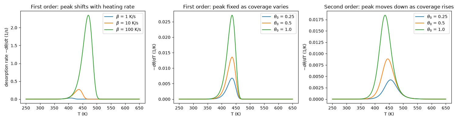First-order peaks shift with heating rate but not with coverage, while second-order peaks move to lower temperature as the coverage rises.

import matplotlib.pyplot as plt

from chemistrykit.surface.systems.tpd import first_order_peak_temperature, redhead_desorption_energy, simulate_tpd

Ed, nu = 110.0e3, 1.0e13  # J/mol, 1/s
for beta in [1.0, 10.0, 100.0]:
    res = simulate_tpd(Ed, nu, beta, T_start=250.0, T_end=650.0)
    Ed_redhead = redhead_desorption_energy(res.peak_temperature, nu, beta)
    print(
        f"beta = {beta:5.1f} K/s: T_p = {res.peak_temperature:.2f} K "
        f"(exact {first_order_peak_temperature(Ed, nu, beta):.2f} K), "
        f"Redhead E_d = {Ed_redhead / 1e3:.2f} kJ/mol (true {Ed / 1e3:.0f})"
    )

beta =   1.0 K/s: T_p = 407.53 K (exact 407.53 K), Redhead E_d = 109.46 kJ/mol (true 110)
beta =  10.0 K/s: T_p = 436.65 K (exact 436.65 K), Redhead E_d = 109.17 kJ/mol (true 110)
beta = 100.0 K/s: T_p = 470.08 K (exact 470.08 K), Redhead E_d = 108.82 kJ/mol (true 110)

fig, axes = plt.subplots(1, 3, figsize=(15, 4))
for beta in [1.0, 10.0, 100.0]:
    res = simulate_tpd(Ed, nu, beta, T_start=250.0, T_end=650.0)
    axes[0].plot(res.T, res.desorption_rate * beta, label=rf"$\beta$ = {beta:g} K/s")
axes[0].set_xlabel("T (K)")
axes[0].set_ylabel(r"desorption rate $-d\theta/dt$ (1/s)")
axes[0].set_title("First order: peak shifts with heating rate")
axes[0].legend()

for theta0 in [0.25, 0.5, 1.0]:
    res = simulate_tpd(Ed, nu, 10.0, theta0=theta0, T_start=250.0, T_end=650.0)
    axes[1].plot(res.T, res.desorption_rate, label=rf"$\theta_0$ = {theta0}")
    res2 = simulate_tpd(Ed, nu, 10.0, theta0=theta0, order=2, T_start=250.0, T_end=650.0)
    axes[2].plot(res2.T, res2.desorption_rate, label=rf"$\theta_0$ = {theta0}")
axes[1].set_title("First order: peak fixed as coverage varies")
axes[2].set_title("Second order: peak moves down as coverage rises")
for ax in axes[1:]:
    ax.set_xlabel("T (K)")
    ax.set_ylabel(r"$-d\theta/dT$ (1/K)")
    ax.legend()
plt.tight_layout()
plt.show()