Clapeyron’s ideal gas law, PV = RT

Clapeyron’s 1834 combined gas law unites Boyle’s law (\(PV\) constant at fixed \(T\)), Charles’s and Gay-Lussac’s law (\(V \propto T\) at fixed \(P\)), and Avogadro’s hypothesis into \(PV_m = RT\). This example draws both classic views with IdealGas: hyperbolic Boyle isotherms, and straight Charles isobars that all extrapolate to zero volume at absolute zero.

import matplotlib.pyplot as plt
import numpy as np

from chemistrykit.thermo.systems.equations_of_state import IdealGas

gas = IdealGas()

fig, axes = plt.subplots(1, 2, figsize=(11, 4.5))

Vm = np.linspace(0.005, 0.05, 300)  # m^3/mol
for T in [200.0, 300.0, 400.0, 500.0]:
    axes[0].plot(Vm * 1000.0, gas.pressure(Vm, T) / 1000.0, label=f"T = {T:.0f} K")
axes[0].set_xlabel(r"$V_m$ (L/mol)")
axes[0].set_ylabel("P (kPa)")
axes[0].set_title("Boyle isotherms: P proportional to 1/V")
axes[0].legend()

T = np.linspace(0.0, 500.0, 200)
for P in [50e3, 101325.0, 200e3]:
    axes[1].plot(T - 273.15, gas.molar_volume(P, np.maximum(T, 1e-9)) * 1000.0, label=f"P = {P / 1000:.0f} kPa")
axes[1].axvline(-273.15, color="gray", linestyle=":")
axes[1].set_xlabel("t (degC)")
axes[1].set_ylabel(r"$V_m$ (L/mol)")
axes[1].set_title("Charles isobars: V extrapolates to 0 at -273.15 degC")
axes[1].legend()
fig.tight_layout()

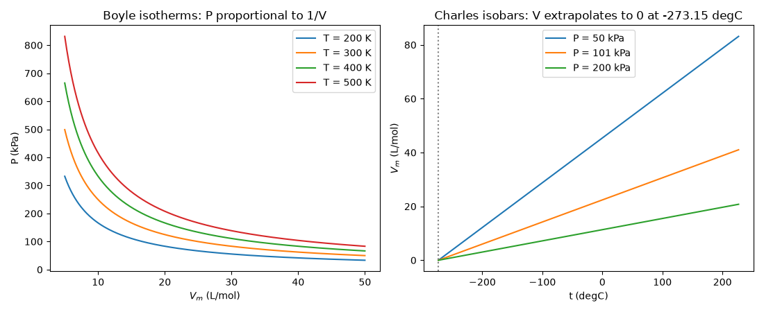
The same law gives the textbook molar volume at 0 degC and 1 atm, and the product \(PV_m\) along any isotherm is the constant \(RT\):

print(f"Vm(273.15 K, 101325 Pa) = {gas.molar_volume(101325.0, 273.15) * 1000.0:.3f} L/mol")
PV = gas.pressure(Vm, 300.0) * Vm
print(f"PV_m along the 300 K isotherm: min {PV.min():.3f}, max {PV.max():.3f} J/mol (= RT = {gas.R * 300.0:.3f})")

plt.show()

Vm(273.15 K, 101325 Pa) = 22.414 L/mol
PV_m along the 300 K isotherm: min 2494.339, max 2494.339 J/mol (= RT = 2494.339)