Cloud-chamber tracks: the positron and the muon

A charged particle in a magnetic field traces a circular arc of radius \(r=p_T/(qB)\). Anderson (1932) used exactly this geometry to identify the positron from a single cloud-chamber photograph: a track curving the “wrong” way for an electron or proton moving in the direction its ionization required. Four years later, Anderson and Neddermeyer (and independently Street and Stevenson) found tracks implying a mass between the electron’s and the proton’s – the muon, identified from the same curvature-plus-ionization method. This example builds both tracks with charged_track_points() and animate_detector_event(), and shows how the arc radius alone fixes momentum, while momentum together with an independent speed estimate is what actually fixes mass.

import matplotlib.pyplot as plt
import numpy as np

from physicskit.particle.kinematics import FourVector
from physicskit.particle.visualizers import animate_detector_event

The arc geometry: r = p_T / (qB)

A positron and an electron with the same momentum, in the same field, curve in opposite senses – exactly the sign-of-charge determination Anderson made from one photograph after a lead plate fixed the direction of travel.

B = 1.0
p_transverse = 2.0
m_e = 0.511e-3  # GeV, so p_transverse (GeV) dominates -- ultrarelativistic, as in a real cloud chamber
E = np.sqrt(p_transverse**2 + m_e**2)
p_positron = FourVector(E, p_transverse, 0.0, 0.0)
p_electron = FourVector(E, p_transverse, 0.0, 0.0)

anim1 = animate_detector_event([p_positron, p_electron], charges=[+1.0, -1.0], B=B)

print("positron and electron, identical momentum, opposite charge:")
print("-> identical curvature radius, opposite sense of bending (exactly Anderson's 1932 observation)")

positron and electron, identical momentum, opposite charge:
-> identical curvature radius, opposite sense of bending (exactly Anderson's 1932 observation)

Momentum from curvature; mass needs an independent speed estimate

The radius r=p_T/(qB) fixes momentum alone – it says nothing about mass by itself, since a fast light particle and a slow heavy one can share the same momentum and hence the same curvature radius. Anderson and Neddermeyer’s muon identification needed a second, independent measurement (ionization density, or penetration through a known absorber thickness in Street and Stevenson’s apparatus) to convert a measured momentum into an inferred mass – exactly what distinguished the muon from both the electron and the proton.

masses_and_labels = [(0.511, "electron"), (105.658, "muon"), (938.272, "proton")]
print("\nsame momentum (p=200 MeV/c), three different masses -> three different speeds (beta):")
for m, label in masses_and_labels:
    p = 200.0
    E = np.sqrt(p**2 + m**2)
    beta = p / E
    print(f"  {label:10s} (m={m:8.3f} MeV): beta = {beta:.6f}  (same curvature radius, very different ionization/penetration)")

fig, ax = plt.subplots(figsize=(6.5, 4.5))
p_range = np.linspace(10.0, 2000.0, 300)
for m, label in masses_and_labels:
    beta = p_range / np.sqrt(p_range**2 + m**2)
    ax.plot(p_range, beta, label=label)
ax.set_xlabel("momentum p (MeV/c)")
ax.set_ylabel(r"speed $\beta = p/E$")
ax.set_title("Same momentum (same curvature), different speed by mass")
ax.legend()
fig.tight_layout()

plt.show()

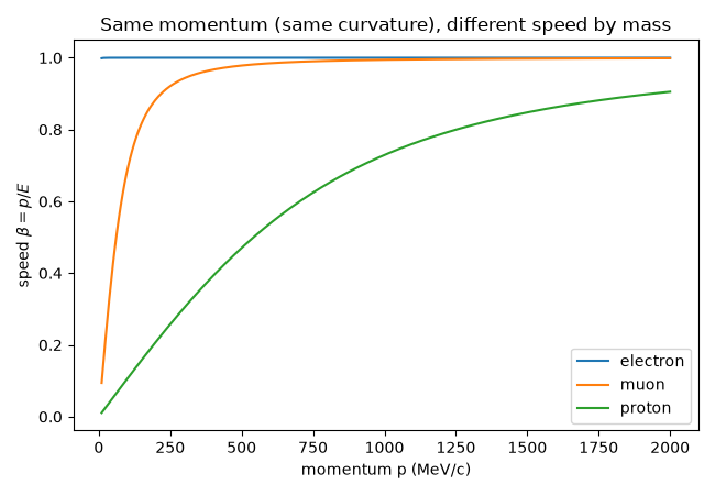
same momentum (p=200 MeV/c), three different masses -> three different speeds (beta):
  electron   (m=   0.511 MeV): beta = 0.999997  (same curvature radius, very different ionization/penetration)
  muon       (m= 105.658 MeV): beta = 0.884198  (same curvature radius, very different ionization/penetration)
  proton     (m= 938.272 MeV): beta = 0.208474  (same curvature radius, very different ionization/penetration)