Examples#
This gallery walks through every physical regime in physicskit.fluids:
inviscid potential flow, classic viscous exact solutions, point-vortex
N-body dynamics, the Kelvin-Helmholtz and Rayleigh-Taylor instabilities,
1D compressible shocks, and the 2D incompressible Navier-Stokes solver that
underlies the instability and turbulence-spectrum tools. Each script
reproduces the signature observable of a specific breakthrough in
Breakthroughs in Fluid Dynamics.
Each script in this gallery is self-contained and can be run directly with
python examples/fluids/<section>/<script>.py. Every script also carries
an RST module docstring as its title/description and uses # %% markers
to split narrative text from code, which is exactly what Sphinx-Gallery
renders into the pages below – the script is the source of truth for what
you see, not a copy of it.
Sections#
potential_flow – inviscid, irrotational flow built by superposing elementary solutions: source, sink, and doublet streamline patterns, d’Alembert’s zero-drag paradox for a circulation-free cylinder, and the classic lifting-cylinder problem with the Kutta-Joukowski lift compared against a direct pressure-integral calculation.
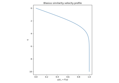
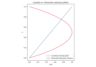
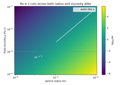
viscous_flow – classic exact viscous solutions: Couette and Poiseuille flow profiles side by side, Stokes drag on a settling sphere, the Reynolds number as the single dimensionless ratio governing flow regime regardless of size or fluid, and the Blasius boundary layer solved by shooting.
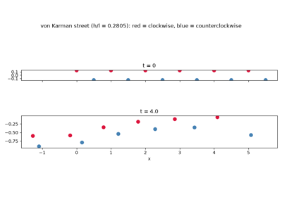
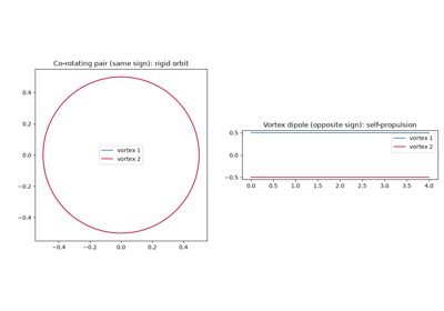
vortex_dynamics – point-vortex N-body dynamics via the Biot-Savart law: a co-rotating vortex pair versus a translating vortex dipole, and a von Karman vortex street holding its staggered shape at the stable spacing ratio.
instabilities – the Kelvin-Helmholtz shear instability rolling a rippled interface into vortex cores, and the Rayleigh-Taylor instability growing a heavy-over-light interface into mushroom plumes, each checked against its linear growth-rate law.
compressible_flow – the 1D Euler equations: normal shock relations across a range of Mach numbers, and the classic Sod shock tube resolving a rarefaction fan, contact discontinuity, and shock in one Riemann problem.
navier_stokes – the 2D incompressible vorticity-streamfunction solver: viscous decay of a periodic vortex patch, Richardson’s cascade, and forced, statistically steady turbulence whose energy spectrum is checked against Kolmogorov’s -5/3 law.
convection – Rayleigh-Bénard convection: the onset for rigid and stress-free walls, growth rates, and the heat flux of convection rolls.
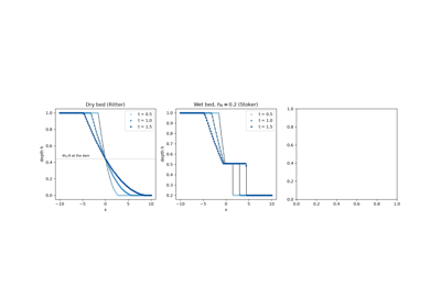
shallow_water – the Saint-Venant equations: the dam break against its exact solution, and Rossby’s geostrophic adjustment.
continuum_mechanics – linear continuum mechanics beyond flow: Fourier’s heat equation (explicit, Crank-Nicolson, and spectral), standing sound waves in pipes and rooms, and Lamé’s pressurized thick-walled cylinder by plane-strain finite elements.
lattice_boltzmann – the D2Q9 BGK lattice Boltzmann method: Poiseuille flow measuring the viscosity law \(\nu = c_s^2(\tau - 1/2)\), and a vortex street shed behind a cylinder.
Compressible Flow#
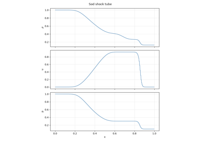
Once a flow moves fast enough that the fluid can no longer get out of its own way, incompressible potential and viscous flow stop applying entirely: the 1D Euler equations support genuinely discontinuous solutions that no smooth velocity field can produce. The normal-shock example sweeps the upstream Mach number through the exact Rankine-Hugoniot jump relations, showing a supersonic flow is always driven back to subsonic on the other side of a shock, at the cost of a sharp pressure and density jump. The Sod shock tube then resolves that same jump dynamically, from a simple burst initial condition, alongside the two other waves – a rarefaction fan and a contact discontinuity – that a general compressible flow problem produces alongside a shock. Watch, in the shock-tube profiles, how a first-order finite-volume scheme smears the shock over several cells even as it gets its speed and downstream state right.
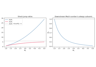
Normal shock relations across a range of Mach numbers
Continuum Mechanics#
Linear continuum mechanics beyond flow. Fourier’s heat equation smooths a temperature field mode by mode. The explicit, Crank-Nicolson, and spectral solvers show how stability and accuracy trade off. Sound in a pipe or a room rings at a discrete set of standing-wave frequencies, recovered here from a single pressure pulse. A pressurized thick-walled cylinder, solved with plane-strain finite elements, reproduces Lamé’s closed-form stresses.
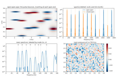
Sound in pipes and rooms: standing modes from a single pulse
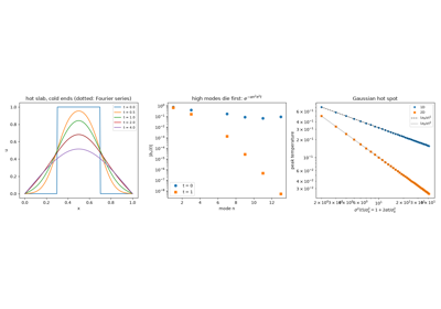
Fourier’s heat equation: every mode decays on its own
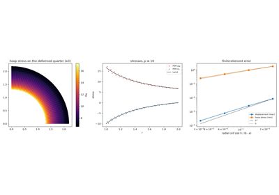
Lamé’s thick-walled cylinder: plane-strain finite elements
Convection#
Rayleigh-Bénard convection in a layer heated from below: the linear onset of convection for stress-free and rigid walls, and the nonlinear convection rolls that carry heat above it.
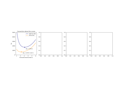
Rayleigh-Bénard convection: the onset at a critical Rayleigh number
Instabilities#
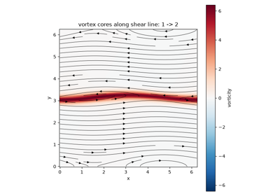
Some flows are unstable to any perturbation, no matter how small: the smallest ripple grows exponentially until it reorganizes the whole flow. Kelvin-Helmholtz instability needs nothing but shear – two layers sliding past each other supply their own energy to grow a ripple into a row of rolled-up vortex cores, the mechanism behind everything from billow clouds to a flapping flag. Rayleigh-Taylor instability needs nothing but an unstable density stratification – heavy fluid sitting on light fluid under gravity – and grows a rippled interface into the mushroom-shaped plumes seen in everything from a lava lamp to a supernova remnant. Both examples below compare the simulated early-time growth against the exact linear growth-rate law for that instability, then run well past the point where that linear theory stops applying, into the fully rolled-up nonlinear state.
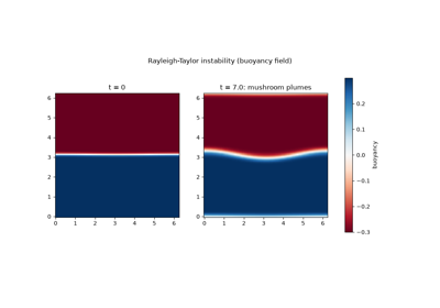
Rayleigh-Taylor plumes from a heavy-over-light interface
Lattice Boltzmann#
A kinetic route to the Navier-Stokes equations. Instead of discretizing the equations of fluid motion, the D2Q9 lattice Boltzmann method moves populations of fictitious particles along nine lattice directions and relaxes them toward a local equilibrium. The viscosity is set entirely by the relaxation time, \(\nu = c_s^2(\tau - 1/2)\). Here it reproduces Poiseuille’s parabola and sheds a vortex street behind a cylinder.
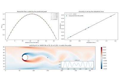
The lattice Boltzmann method: Navier-Stokes from colliding populations
Navier-Stokes and Turbulence#
The general-purpose engine behind this package’s instability simulations: a doubly periodic, pseudo-spectral solver for the full 2D incompressible vorticity-transport equation, exact up to machine precision and aliasing in space and 4th-order accurate in time. The first example shows its most basic signature – a vortex patch’s peak vorticity bleeding away under viscous diffusion, at a rate no inviscid simulation could reproduce. Another follows Richardson’s qualitative cascade – a few large eddies folding into ever finer filaments until viscosity takes over. The last adds steady random forcing and a large-scale drag, so that the flow reaches a statistically steady state with a constant energy flux through the scales. Its time-averaged energy spectrum follows Kolmogorov’s predicted -5/3 power law over the range between the forcing scale and the drag scale.
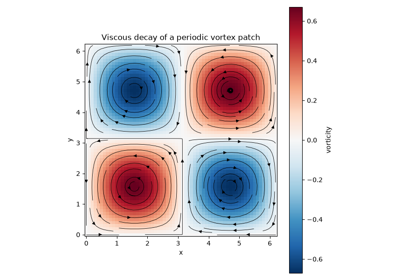
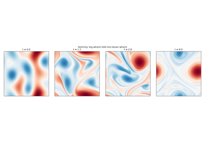
Richardson’s cascade: big whorls have little whorls
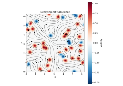
The Kolmogorov -5/3 cascade in forced 2D turbulence
Potential Flow#
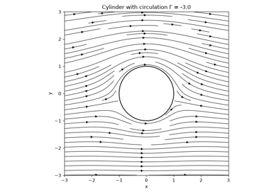
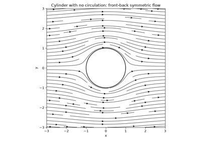
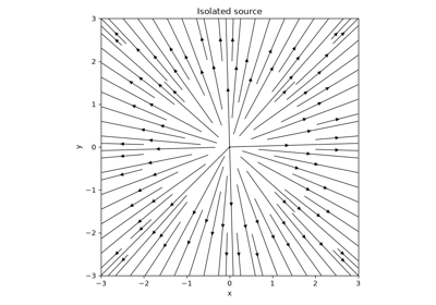
Away from any boundary layer or wake, a great deal of real aerodynamics is governed by a flow with no vorticity at all: a velocity potential obeying Laplace’s equation, which is linear, so entire flow fields can be built by just adding together a handful of elementary solutions. The examples below build up from Bernoulli’s pressure-speed trade-off and a bare source/sink/doublet, through d’Alembert’s paradox of exactly zero drag on a circulation-free cylinder, to the textbook result that made potential theory indispensable to early aerodynamics – a spinning cylinder, or by extension a cambered airfoil, generates lift in direct proportion to its bound circulation, with no viscosity anywhere in the calculation. Watch, in the streamline plots, how a source and sink merge into a doublet as they’re brought together, and how adding circulation to a symmetric cylinder flow breaks its front-back symmetry and shifts its stagnation points – the geometric signature of lift.
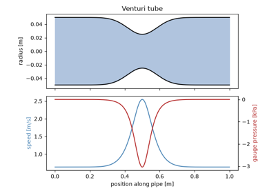
Bernoulli’s principle: faster flow, lower pressure
The Kutta-Joukowski lift theorem: a cylinder with circulation
D’Alembert’s paradox: zero net drag on a cylinder in inviscid flow
Source, sink, and doublet: building blocks of potential flow
Shallow Water#
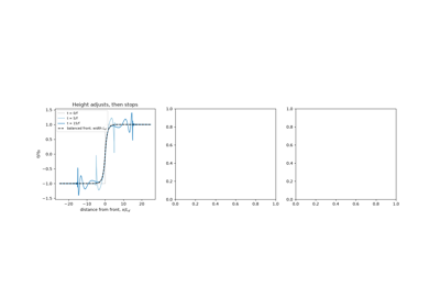
The Saint-Venant shallow-water equations: a dam break solved numerically and compared with its exact solution, and Rossby’s geostrophic adjustment of a height front on a rotating planet.
Rossby’s geostrophic adjustment: a front that does not spread
Viscous Flow#
Viscosity is what potential flow leaves out, and these are the handful of problems simple enough that adding it back in still yields an exact, closed-form answer. Couette and Poiseuille flow show how the same viscous term produces a straight-line profile under a moving wall but a parabola under a pressure gradient; Stokes drag captures the opposite extreme, where viscosity so dominates inertia that a settling sphere never notices its own momentum; the Reynolds number sweep shows that same Stokes-drag physics recast to make a different point – that a single dimensionless ratio, not the sphere’s size or the fluid’s identity separately, decides the flow regime; and the Blasius boundary layer shows what happens in between – a thin viscous layer clinging to a wall in an otherwise fast, nearly inviscid stream, thickening as the square root of downstream distance. Watch how thin that layer stays even at a middling free-stream speed, and how the wall shear stress it predicts falls off as the flow moves downstream.
The Reynolds number: one ratio, regardless of size or fluid
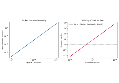
Stokes drag and the terminal velocity of a settling sphere
Vortex Dynamics#
Concentrate all of a flow’s vorticity into a handful of points and the Navier-Stokes equations collapse to ordinary differential equations: each point vortex simply drifts in the velocity field induced by every other one. The examples below show how differently two vortices behave depending only on the relative sign of their circulation – a rigid, orbiting pair if the signs match, a self-propelling dipole that runs off in a straight line if they don’t – and then scale that same Biot-Savart mechanics up to a full von Karman street, the staggered double row shed behind every bluff body from a chimney to a violin string in the wind. Watch how the street holds its staggered spacing intact at von Karman’s stable ratio, in stark contrast to the pairwise dynamics of the first example.