The Saint-Venant equations: a dam break

Saint-Venant’s shallow-water equations (1871) describe flows much wider than they are deep, such as rivers, tides, tsunamis and floods, by the depth \(h\) and the depth-averaged velocity \(u\) alone:

\[\partial_t h + \partial_x(hu) = 0, \qquad \partial_t(hu) + \partial_x\left(hu^2 + \tfrac12 gh^2\right) = 0.\]

Waves travel at \(c = \sqrt{gh}\), and steep fronts become bores, the shocks of this system. The dam break, a reservoir of depth \(h_L\) released at \(t = 0\) into tailwater of depth \(h_R\), has an exact solution: a rarefaction fan running back into the reservoir and a bore running forward (Ritter 1892 for a dry bed, Stoker 1957 for a wet one). At the dam site the depth is \(4h_L/9\) for a dry bed, whatever the time. This example solves both cases with a finite-volume HLL scheme and compares with the exact profiles.

import matplotlib.pyplot as plt
import numpy as np

from physicskit.fluids.systems.shallow_water import dam_break_exact, shallow_water_1d

g = 9.81
h_left = 1.0
x = np.linspace(-10.0, 10.0, 801)
times = [0.5, 1.0, 1.5]

fig, axes = plt.subplots(1, 3, figsize=(15, 4))
errors = {}
for ax, h_right, title in [(axes[0], 0.0, "Dry bed (Ritter)"), (axes[1], 0.2, r"Wet bed, $h_R = 0.2$ (Stoker)")]:
    for t, color in zip(times, ["#9ecae1", "#4292c6", "#08519c"]):
        num = shallow_water_1d(np.where(x < 0, h_left, h_right), np.zeros_like(x), x, t_max=t, g=g)
        h_exact, _ = dam_break_exact(x, t, h_left, h_right, g)
        ax.plot(x, h_exact, "k-", lw=1)
        ax.plot(x[::8], num["h"][::8], "o", ms=3, color=color, label=f"t = {t}")
        errors[(h_right, t)] = np.mean(np.abs(num["h"] - h_exact))
    ax.set_xlabel("x")
    ax.set_ylabel("depth h")
    ax.set_title(title)
    ax.legend()
axes[0].axhline(4 * h_left / 9, color="gray", ls=":", lw=1)
axes[0].text(-9.5, 4 * h_left / 9 + 0.02, r"$4h_L/9$ at the dam", fontsize=8)

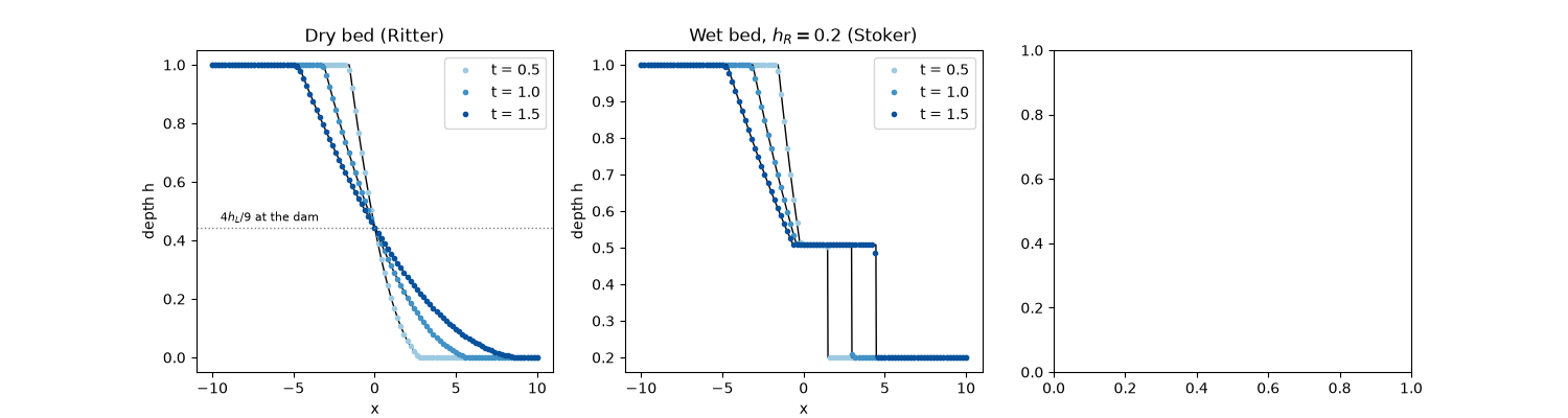
Text(-9.5, 0.46444444444444444, '$4h_L/9$ at the dam')

Bore height and speed against tailwater depth

The exact solution’s middle state, read off the profile, shows the bore growing in height but slowing down as the tailwater gets shallower.

hr_values = np.linspace(0.02, 0.8, 30)
bore_height, bore_speed = [], []
for hr in hr_values:
    xs = np.linspace(-5, 15, 40001)
    h, _ = dam_break_exact(xs, 1.0, h_left, hr, g)
    j = np.argmax(np.abs(np.diff(h)))
    bore_height.append(h[j] - hr)
    bore_speed.append(xs[j + 1])
axes[2].plot(hr_values, bore_height, color="navy", label=r"bore height $h_m - h_R$")
ax2 = axes[2].twinx()
ax2.plot(hr_values, np.array(bore_speed) / np.sqrt(g * h_left), color="crimson", label=r"bore speed $s / c_L$")
ax2.axhline(2.0, color="crimson", ls=":", lw=1)
axes[2].set_xlabel(r"tailwater depth $h_R / h_L$")
axes[2].set_ylabel("bore height", color="navy")
ax2.set_ylabel(r"$s / \sqrt{g h_L}$ (dry front: 2)", color="crimson")
axes[2].set_title("Stoker's bore")
plt.tight_layout()
plt.show()
for key, err in errors.items():
    print(f"h_R = {key[0]}, t = {key[1]}: mean |h - h_exact| = {err:.2e}")

h_R = 0.0, t = 0.5: mean |h - h_exact| = 6.75e-04
h_R = 0.0, t = 1.0: mean |h - h_exact| = 6.76e-04
h_R = 0.0, t = 1.5: mean |h - h_exact| = 6.77e-04
h_R = 0.2, t = 0.5: mean |h - h_exact| = 7.53e-04
h_R = 0.2, t = 1.0: mean |h - h_exact| = 6.94e-04
h_R = 0.2, t = 1.5: mean |h - h_exact| = 8.11e-04

Check

assert max(errors.values()) < 2e-3
num = shallow_water_1d(np.where(x < 0, h_left, 0.0), np.zeros_like(x), x, t_max=1.0, g=g)
assert abs(num["h"][np.argmin(np.abs(x))] - 4 * h_left / 9) < 5e-3