Rossby’s geostrophic adjustment: a front that does not spread

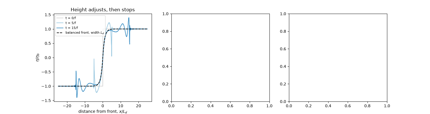
Without rotation, a step in the height of a shallow layer collapses completely, radiating its energy away as gravity waves. Rossby (1938) showed that on a rotating planet it does not. The linear rotating shallow-water equations

\[\partial_t u - fv = -g\partial_x\eta, \qquad \partial_t v + fu = 0, \qquad \partial_t\eta + H\partial_x u = 0\]

conserve the potential vorticity \(q = \partial_x v - f\eta/H\) at each point. The flow therefore cannot relax to a flat surface, and only part of the step’s energy leaves as inertia-gravity waves of frequency \(\sqrt{f^2 + gHk^2}\). What remains is a front in geostrophic balance, \(fv = g\partial_x\eta\),

\[\eta = \eta_0\,\mathrm{sgn}(x)\left(1 - e^{-|x|/L_d}\right), \qquad L_d = \frac{\sqrt{gH}}{f},\]

with a jet along it and the Rossby radius of deformation \(L_d\) as its width. That length sets the size of weather systems and ocean eddies. This example evolves the problem exactly, mode by mode, on a periodic domain holding two opposite fronts.

import matplotlib.pyplot as plt
import numpy as np

from physicskit.fluids.systems.shallow_water import geostrophic_adjustment_steady, rotating_shallow_water_1d

g, H, f = 1.0, 1.0, 1.0
L_d = np.sqrt(g * H) / f
L = 200.0
x = np.linspace(-L / 2, L / 2, 2048, endpoint=False)
eta0 = np.where(np.abs(x) < L / 4, 1.0, -1.0)

times = np.linspace(0.0, 300.0, 3001)
out = rotating_shallow_water_1d(eta0, x, times, g, H, f)
steady = geostrophic_adjustment_steady(eta0, x, g, H, f)

Snapshots around the front at x = -L/4

fig, axes = plt.subplots(1, 3, figsize=(15, 4))
view = np.abs(x + L / 4) < 25
for t, color in [(0.0, "lightgray"), (5.0, "#9ecae1"), (15.0, "#4292c6")]:
    i = np.argmin(np.abs(times - t))
    axes[0].plot(x[view] + L / 4, out["eta"][i, view], color=color, label=f"t = {t:g}/f")
xi = x[view] + L / 4
axes[0].plot(xi, np.sign(xi) * (1 - np.exp(-np.abs(xi) / L_d)), "k--", label=r"balanced front, width $L_d$")
axes[0].set_xlabel(r"distance from front, $x / L_d$")
axes[0].set_ylabel(r"$\eta / \eta_0$")
axes[0].set_title("Height adjusts, then stops")
axes[0].legend(fontsize=8)

<matplotlib.legend.Legend object at 0x130f6fbf0>

The time-mean state is the balanced one

late = times > 100.0
eta_mean = out["eta"][late].mean(axis=0)
v_mean = out["v"][late].mean(axis=0)
axes[1].plot(xi, eta_mean[view], color="navy", label=r"time-mean $\eta$")
axes[1].plot(xi, steady["eta"][view], "k--", lw=1, label="PV inversion")
axes[1].plot(xi, v_mean[view], color="crimson", label="time-mean jet $v$")
axes[1].plot(xi, steady["v"][view], "k:", lw=1, label=r"$v = (g/f)\,\partial_x\eta$")
axes[1].set_xlabel(r"$x / L_d$")
axes[1].set_title("Geostrophic balance")
axes[1].legend(fontsize=8)

<matplotlib.legend.Legend object at 0x132a9bd70>

Energy: only part of it radiates away

For an infinite step, the balanced state keeps exactly a third of the potential energy released, the rest leaving in inertia-gravity waves (Gill 1982, sec. 7.3).

dx = x[1] - x[0]
PE0 = 0.5 * g * np.sum(eta0**2) * dx
PE_released = 0.5 * g * np.sum(eta0**2 - steady["eta"] ** 2) * dx
KE_balanced = 0.5 * H * np.sum(steady["v"] ** 2) * dx
wave_energy = 0.5 * np.sum(H * (out["u"] ** 2 + (out["v"] - steady["v"]) ** 2) + g * (out["eta"] - steady["eta"]) ** 2, axis=1) * dx
axes[2].plot(times, wave_energy / PE_released, color="navy", label="inertia-gravity waves")
axes[2].axhline(KE_balanced / PE_released, color="crimson", label="balanced jet")
axes[2].axhline(2 / 3, color="gray", ls=":", lw=1)
axes[2].axhline(1 / 3, color="gray", ls=":", lw=1)
axes[2].set_ylim(0, 1)
axes[2].set_xlabel("t f")
axes[2].set_ylabel("fraction of released potential energy")
axes[2].set_title(f"Kept in balance: {KE_balanced / PE_released:.3f}")
axes[2].legend()
plt.tight_layout()
plt.show()
print(f"Rossby radius L_d = {L_d}; balanced fraction {KE_balanced / PE_released:.4f} (exact 1/3)")

Rossby radius L_d = 1.0; balanced fraction 0.3337 (exact 1/3)

Check

the discrete step sits half a cell to the right of x = -L/4

front = x + L / 4 - dx / 2
near = np.abs(front) < 20
exact = np.sign(front) * (1 - np.exp(-np.abs(front) / L_d))
np.testing.assert_allclose(steady["eta"][near], exact[near], atol=0.02)
np.testing.assert_allclose(eta_mean, steady["eta"], atol=0.01)
assert abs(KE_balanced / PE_released - 1 / 3) < 0.01