The lattice Boltzmann method: Navier-Stokes from colliding populations

Lattice gas automata (Frisch, Hasslacher and Pomeau, 1986) showed that Boolean particles hopping and colliding on a hexagonal lattice obey the Navier-Stokes equations on large scales. They were noisy, though. The lattice Boltzmann method (McNamara and Zanetti, 1988) replaced the particles with their average populations \(f_i\), one per lattice direction. Qian, d’Humières and Lallemand (1992) reduced the collisions to a single relaxation toward a local equilibrium, the BGK operator:

\[f_i(\mathbf x + \mathbf e_i, t + 1) = f_i - \frac{1}{\tau}\left(f_i - f_i^{\rm eq}\right).\]

In the resulting fluid, the relaxation time alone sets the viscosity, \(\nu = c_s^2(\tau - \tfrac12)\) with \(c_s^2 = 1/3\).

This example uses LatticeBoltzmannD2Q9 to check that relation in a body-force-driven channel against Poiseuille’s parabola, and then to shed a von Kármán vortex street behind a cylinder. Everything is in lattice units.

import matplotlib.pyplot as plt
import numpy as np

from physicskit.fluids import LatticeBoltzmannD2Q9, lbm_viscosity, poiseuille_flow_velocity

Poiseuille flow and the viscosity law

A periodic channel of width \(H = 32\) between two walls, placed by bounce-back halfway between the last fluid and first solid node, is driven by a uniform acceleration \(g\). The steady profile is \(u = g\,y(H - y)/2\nu\), so its peak measures the viscosity.

ny, g = 34, 1e-6
H = ny - 2
y = np.arange(ny) - 0.5
solid = np.zeros((1, ny), dtype=bool)
solid[:, [0, -1]] = True
taus = [0.6, 0.5 + np.sqrt(3 / 16), 1.0, 1.5]
profiles, nu_fit = {}, []
for tau in taus:
    lb = LatticeBoltzmannD2Q9(1, ny, tau, body_force=(g, 0.0), solid=solid)
    lb.step(int(3 * H**2 / lb.viscosity))
    u = lb.velocity[0][0, 1:-1]
    profiles[tau] = u
    # least-squares fit of u = (g / 2 nu) y (H - y) for nu
    shape = y[1:-1] * (H - y[1:-1]) * g / 2
    nu_fit.append(np.sum(shape * shape) / np.sum(shape * u))
    print(f"tau = {tau:.3f}: nu from the profile {nu_fit[-1]:.5f}, (tau - 1/2)/3 = {lbm_viscosity(tau):.5f}")

tau = 0.600: nu from the profile 0.03337, (tau - 1/2)/3 = 0.03333
tau = 0.933: nu from the profile 0.14434, (tau - 1/2)/3 = 0.14434
tau = 1.000: nu from the profile 0.16660, (tau - 1/2)/3 = 0.16667
tau = 1.500: nu from the profile 0.33158, (tau - 1/2)/3 = 0.33333

At \(\tau = 1/2 + \sqrt{3/16} \approx 0.933\) the BGK bounce-back wall sits exactly halfway and the parabola is reproduced to round-off. At other values of \(\tau\) a small slip remains.

A vortex street behind a cylinder

A cylinder of diameter \(D = 20\) in the same kind of channel, now periodic along 320 nodes, with \(\tau = 0.55\). Above a Reynolds number of about 50, the wake stops being steady and alternately sheds vortices from each side. A probe downstream records the cross-flow velocity, and its frequency gives the Strouhal number \(St = fD/U\). The walls confine the wake (the cylinder blocks a quarter of the channel), which raises \(St\) above the value of about 0.14 for an unbounded cylinder at this Reynolds number.

nx, ny, D, tau = 320, 82, 20, 0.55
X, Y = np.meshgrid(np.arange(nx), np.arange(ny), indexing="ij")
body = (X - 70) ** 2 + (Y - 42.5) ** 2 <= (D / 2) ** 2  # one node off-center, to trigger shedding
walls = np.zeros_like(body)
walls[:, [0, -1]] = True
nu = lbm_viscosity(tau)
U0 = 0.08
lb = LatticeBoltzmannD2Q9(nx, ny, tau, body_force=(1.6 * 12 * nu * U0 / (ny - 2) ** 2, 0.0), solid=body | walls, velocity=(U0, 0.0))
lb.step(6000)
probe, speed = [], []
for _ in range(200):
    lb.step(50)
    ux, uy = lb.velocity
    probe.append(uy[150, 42])
    speed.append(ux[~(body | walls)].mean())
probe = np.array(probe)
t_probe = 6000 + 50 * np.arange(1, 201)
U = np.mean(speed)
spec = np.abs(np.fft.rfft((probe - probe.mean()) * np.hanning(len(probe)), 8 * len(probe)))
freqs = np.fft.rfftfreq(8 * len(probe), 50)
f_shed = freqs[np.argmax(spec)]
print(f"mean speed U = {U:.4f}, Re = U D / nu = {U * D / nu:.0f}")
print(f"shedding frequency {f_shed:.2e} per step, Strouhal number St = f D / U = {f_shed * D / U:.2f}")

fig = plt.figure(figsize=(15, 8))
ax1 = fig.add_subplot(2, 2, 1)
for tau, u in profiles.items():
    ax1.plot(y[1:-1], u / (g * H**2 / (8 * lbm_viscosity(tau))), "o", ms=3, label=rf"$\tau$ = {tau:.3f}")
ax1.plot(y[1:-1], poiseuille_flow_velocity(y[1:-1], -1.0, 1.0, H) / (H**2 / 8), "k-", lw=1, label="parabola")
ax1.set_xlabel("distance from the wall y")
ax1.set_ylabel(r"$u / u_{\max}$")
ax1.set_title("Poiseuille flow, scaled by the predicted peak")
ax1.legend(fontsize=8)

ax2 = fig.add_subplot(2, 2, 2)
tt = np.linspace(0.52, 1.6, 50)
ax2.plot(tt, (tt - 0.5) / 3, "k-", lw=1, label=r"$\nu = (\tau - 1/2)/3$")
ax2.plot(taus, nu_fit, "o", label="measured from the profile")
ax2.set_xlabel(r"relaxation time $\tau$")
ax2.set_ylabel(r"viscosity $\nu$")
ax2.set_title("viscosity is set by the relaxation time")
ax2.legend()

ax3 = fig.add_subplot(2, 2, (3, 4))
w = lb.vorticity()
w[body | walls] = np.nan
im = ax3.imshow(w.T, origin="lower", cmap="RdBu_r", vmin=-0.02, vmax=0.02)
ax3.contour(body.T.astype(float), levels=[0.5], colors="k", linewidths=1)
ax3.plot(150, 42, "k+", ms=10)
ax3.set_title(f"vorticity at t = {lb.time} (Re = {U * D / nu:.0f}, St = {f_shed * D / U:.2f}); + marks the probe")
fig.colorbar(im, ax=ax3, shrink=0.8)
inset = ax3.inset_axes([0.62, 0.06, 0.36, 0.3])
inset.plot(t_probe, probe, lw=0.8)
inset.set_title(r"probe $u_y(t)$", fontsize=8)
inset.tick_params(labelsize=6)
fig.tight_layout()
plt.show()

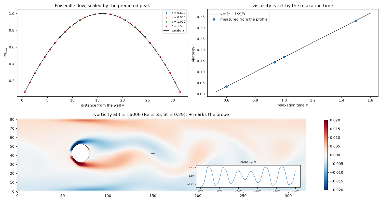
mean speed U = 0.0460, Re = U D / nu = 55
shedding frequency 6.75e-04 per step, Strouhal number St = f D / U = 0.29

Check

BGK viscosity nu = (tau - 1/2)/3 recovered from Poiseuille profiles, and periodic vortex shedding behind the cylinder (Strouhal number of order 0.1-0.3 at this Re and blockage).

np.testing.assert_allclose(nu_fit, [lbm_viscosity(tau_i) for tau_i in taus], rtol=0.01)
assert 0.1 < f_shed * D / U < 0.35
assert spec.max() > 10 * np.median(spec)