Rayleigh-Taylor plumes from a heavy-over-light interface

A denser fluid layer sits atop a lighter one – exactly the unstable arrangement – separated by an interface with a small sinusoidal ripple. The two layers are represented not as a sharp density jump but through the Boussinesq approximation: a dimensionless buoyancy field \(b=-\delta\rho/\rho_0\) (positive where the fluid is locally lighter than the reference density), advected and diffused like vorticity but also exerting a baroclinic torque \(g\,\partial_x b\) on it wherever the density gradient is non-vertical:

\[\partial_t \omega + (\mathbf{u}\cdot\nabla)\omega = \nu \nabla^2 \omega + g\,\partial_x b, \qquad \partial_t b + (\mathbf{u}\cdot\nabla) b = \kappa \nabla^2 b,\]

with \(\mathbf{u}\) recovered from \(\omega\) exactly as in physicskit.fluids.systems.navier_stokes. Rayleigh’s 1883 linear stability analysis (extended by Taylor in 1950) shows that any interface with heavy fluid sitting on light fluid under gravity \(g\) is unconditionally unstable, growing a small ripple of wavenumber \(k\) at rate

\[\sigma(k) = \sqrt{A\,g\,k}, \qquad A = \frac{\rho_{heavy}-\rho_{light}}{\rho_{heavy}+\rho_{light}},\]

where \(A\) is the Atwood number setting the buoyancy jump across the interface. This example builds that heavy-over-light arrangement with rayleigh_taylor_ic(), checks the early growth against rayleigh_taylor_growth_rate(), and then evolves the coupled equations above with simulate_rayleigh_taylor() well into the nonlinear regime, where the interface rolls up into the mushroom-shaped plumes the instability is named for.

import matplotlib.pyplot as plt
import numpy as np

from physicskit.fluids.core.grid import spectral_grid
from physicskit.fluids.systems.instabilities import (
    rayleigh_taylor_growth_rate,
    rayleigh_taylor_ic,
    simulate_rayleigh_taylor,
)
from physicskit.fluids.visualizers.flow_fields import animate_rayleigh_taylor

A rippled heavy-over-light interface

n, length = 96, 2 * np.pi
atwood, g, nu, kappa = 0.3, 1.0, 0.001, 0.001
omega0, buoyancy0 = rayleigh_taylor_ic(n, length, atwood_number=atwood, perturbation_amplitude=0.01)

Grow it and compare against the linear prediction

k0 = 2 * np.pi / length
sigma_predicted = rayleigh_taylor_growth_rate(k=k0, atwood_number=atwood, g=g)

omega, buoyancy = omega0.copy(), buoyancy0.copy()
amps, times = [], []
dt, chunk = 0.01, 50
for i in range(14):
    result = simulate_rayleigh_taylor(omega, buoyancy, nu=nu, kappa=kappa, g=g, dt=dt, steps=chunk, length=length)
    omega, buoyancy = result["omega"], result["buoyancy"]
    dev = buoyancy - buoyancy.mean(axis=0, keepdims=True)
    amps.append(np.sqrt(np.mean(dev**2)))
    times.append((i + 1) * dt * chunk)
amps, times = np.array(amps), np.array(times)
print(f"growth rate: linear theory sigma = {sigma_predicted:.3f}")
print(f"interface roughness grew by a factor of {amps[-1] / amps[0]:.2f} over the run")

growth rate: linear theory sigma = 0.548
interface roughness grew by a factor of 11.62 over the run

The nonlinear mushroom plumes

X, Y, _, _, _ = spectral_grid(n, length)

fig, axes = plt.subplots(1, 2, figsize=(11, 5))
axes[0].pcolormesh(X, Y, buoyancy0, cmap="RdBu", shading="auto")
axes[0].set_title("t = 0")
axes[0].set_aspect("equal")
im1 = axes[1].pcolormesh(X, Y, buoyancy, cmap="RdBu", shading="auto")
axes[1].set_title(f"t = {times[-1]:.1f}: mushroom plumes")
axes[1].set_aspect("equal")
fig.colorbar(im1, ax=axes, label="buoyancy")
fig.suptitle("Rayleigh-Taylor instability (buoyancy field)")

plt.show()

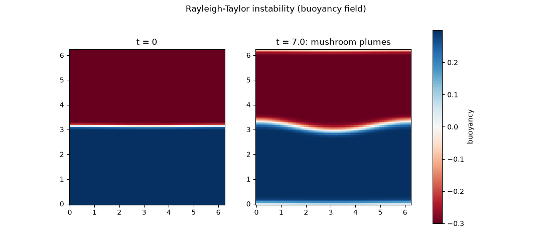
Watching the mushroom plumes form, continuously

Rather than a single before/after comparison, redrawing the buoyancy field every few RK4 steps shows the rippled interface rolling up into the characteristic mushroom-shaped plumes as it happens.

anim = animate_rayleigh_taylor(omega0, buoyancy0, nu=nu, kappa=kappa, g=g, dt=dt, steps_per_frame=chunk, n_frames=20, length=length)

plt.show()