Roll-up of a shear layer into vortex cores

Helmholtz (1868) and Kelvin (1871) showed that any interface between two fluid layers sliding past each other is unconditionally unstable: the shear itself supplies the energy to grow a small ripple, with no velocity threshold required. kelvin_helmholtz_ic() seeds exactly this thin, rippled shear layer as a vorticity field on a doubly periodic domain, and NavierStokes2D evolves it by integrating the 2D incompressible vorticity-transport equation

\[\partial_t \omega + (\mathbf{u}\cdot\nabla)\omega = \nu \nabla^2 \omega\]

(velocity recovered from the streamfunction, \(\nabla^2\psi=-\omega\), \(\mathbf{u}=(\partial_y\psi,\,-\partial_x\psi)\)) through the roll-up – from a single smooth ripple to several discrete “cat’s eye” vortex cores – while the idealized vortex-sheet linear theory,

\[\sigma(k) = \frac{k\,\Delta u}{2}\]

(kelvin_helmholtz_growth_rate()), predicts how fast a perturbation of wavenumber \(k\) should grow, for a velocity jump \(\Delta u\) across the layer, before it does.

import matplotlib.pyplot as plt
import numpy as np
from scipy.signal import find_peaks

from physicskit.fluids.systems.instabilities import kelvin_helmholtz_growth_rate, kelvin_helmholtz_ic
from physicskit.fluids.systems.navier_stokes import NavierStokes2D
from physicskit.fluids.visualizers.flow_fields import animate_kelvin_helmholtz, plot_vorticity_field

A thin vortex sheet with a small sinusoidal ripple seed

n, length = 128, 2 * np.pi
shear_width, amplitude = 0.15, 0.1
omega0 = kelvin_helmholtz_ic(n, length, shear_width=shear_width, perturbation_amplitude=amplitude)
solver = NavierStokes2D(n=n, length=length, nu=0.0005)

Early-time growth versus the linear prediction

The idealized vortex-sheet growth-rate law predicts \(\sigma = k\,\Delta u/2\) for a perturbation of wavenumber k (the shear jump here is \(\Delta u \approx 2\), the tanh profile’s asymptotic jump); it is a lower bound for this finite-thickness layer, whose fastest-growing wavelength is comparable to the shear width itself (Michalke, 1964) rather than to the domain-scale fundamental mode used below, so the measured RMS growth – fed by that shorter, faster-growing wavelength – comes out several times higher than the fundamental-mode estimate.

k0 = 2 * np.pi / length
sigma_predicted = kelvin_helmholtz_growth_rate(k=k0, delta_u=2.0)

omega = omega0.copy()
amps, times = [], []
dt, chunk = 0.002, 25
for i in range(8):
    omega = solver.simulate(omega, dt=dt, steps=chunk)["omega"]
    dev = omega - omega.mean(axis=0, keepdims=True)
    amps.append(np.sqrt(np.mean(dev**2)))
    times.append((i + 1) * dt * chunk)
amps, times = np.array(amps), np.array(times)
sigma_measured = np.polyfit(times[:4], np.log(amps[:4]), 1)[0]
print(f"fundamental-mode lower bound: sigma = {sigma_predicted:.3f}; measured early-time RMS growth rate = {sigma_measured:.3f}")

fundamental-mode lower bound: sigma = 1.000; measured early-time RMS growth rate = 3.943

Full nonlinear roll-up

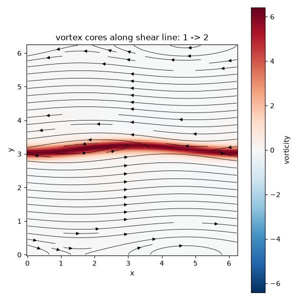
Continuing well past the linear regime rolls the sheet up into discrete “cat’s eye” vortex cores – counting peaks along the (former) shear line makes the roll-up quantitative, not just visual.

for _ in range(20):
    omega = solver.simulate(omega, dt=dt, steps=chunk)["omega"]

row0 = omega0[:, n // 2]
rowf = omega[:, n // 2]
peaks0, _ = find_peaks(row0)
peaksf, _ = find_peaks(rowf)

u, v = solver.velocity(omega)
fig, ax = plot_vorticity_field(solver.X, solver.Y, omega, u, v)
ax.set_title(f"vortex cores along shear line: {len(peaks0)} -> {len(peaksf)}")
fig.tight_layout()

plt.show()

Watching the roll-up happen, continuously

Rather than a single before/after comparison, redrawing the vorticity field every few RK4 steps shows the ripple rolling up into discrete “cat’s eye” vortex cores as it happens.

anim = animate_kelvin_helmholtz(omega0, nu=0.0005, dt=0.002, steps_per_frame=10, n_frames=40, length=length)

plt.show()