Source, sink, and doublet: building blocks of potential flow

For a 2D flow with no vorticity (\(\nabla\times\mathbf{u}=0\)), the velocity is the gradient of a scalar potential, \(\mathbf{u}=\nabla\phi\), and incompressibility (\(\nabla\cdot\mathbf{u}=0\)) then makes \(\phi\) satisfy Laplace’s equation,

\[\nabla^2 \phi = 0.\]

Laplace’s equation is linear, so any two solutions can be added together to make a third. This example builds up the classic progression of elementary solutions, each expressed through its complex potential \(W(z) = \phi + i\psi\) at \(z = x+iy\) (velocity recovered as \(u-iv=dW/dz\)): an isolated source of strength \(m\) (volume flow rate per unit depth),

\[W(z) = \frac{m}{2\pi}\ln(z - z_0),\]

a source-sink pair, and the doublet those two collapse into as their separation shrinks to zero while the product \(\kappa = m\,(\text{separation})\) is held fixed – doublet_potential(), \(W(z) = \kappa/(2\pi(z-z_0))\), is exactly that zero-separation limit, and (as the next example shows) superposing it with a uniform stream is what produces flow past a cylinder.

import matplotlib.pyplot as plt
import numpy as np

from physicskit.fluids.systems.potential_flow import PotentialFlow
from physicskit.fluids.visualizers.flow_fields import plot_streamlines

A single source

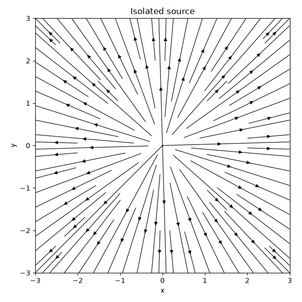
With strength \(m=1\) and no free stream (\(U_\infty=0\)), the flow is pure radial outflow: streamlines radiate straight outward from the source in every direction, with speed falling off as \(m/(2\pi r)\).

x = np.linspace(-3, 3, 200)
X, Y = np.meshgrid(x, x, indexing="ij")

source_flow = PotentialFlow(U_inf=0.0)
source_flow.add_source(strength=1.0)
u, v = source_flow.velocity(X, Y)

fig, ax = plot_streamlines(X, Y, u, v)
ax.set_title("Isolated source")
fig.tight_layout()

A source-sink pair

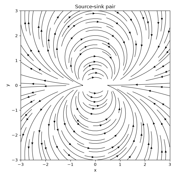
A source of strength \(m=1\) at \(x_0=-0.5\) and a sink (strength=-1) at \(x_0=+0.5\) – the complex potential is just the sum \(W(z) = \frac{m}{2\pi}\ln(z+0.5) - \frac{m}{2\pi}\ln(z-0.5)\). Bringing an equal-strength sink nearby closes the streamlines into loops running from source to sink.

pair_flow = PotentialFlow(U_inf=0.0)
pair_flow.add_source(strength=1.0, x0=-0.5, y0=0.0)
pair_flow.add_source(strength=-1.0, x0=0.5, y0=0.0)
u, v = pair_flow.velocity(X, Y)

fig, ax = plot_streamlines(X, Y, u, v)
ax.set_title("Source-sink pair")
fig.tight_layout()

The doublet limit

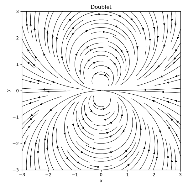
Shrinking the source-sink separation to zero while keeping the product \(\kappa = m\,(\text{separation})\) fixed – here \(\kappa=2\) – is exactly what doublet_potential() computes directly, via \(W(z) = \kappa/(2\pi z)\); the loops above collapse into the doublet’s characteristic circular streamline pattern threading the origin.

doublet_flow = PotentialFlow(U_inf=0.0)
doublet_flow.add_doublet(strength=2.0)
u, v = doublet_flow.velocity(X, Y)

fig, ax = plot_streamlines(X, Y, u, v)
ax.set_title("Doublet")
fig.tight_layout()

Speed and streamfunction together

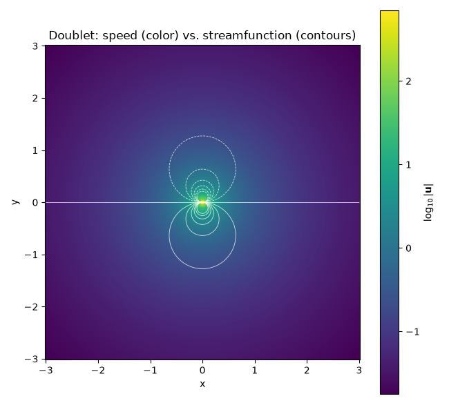
Streamlines alone show direction but not magnitude. The doublet’s speed \(|\mathbf{u}| = \kappa/(2\pi r^2)\) – computed here from the same velocity() call as above – diverges at the singular point and falls off quickly away from it; overlaying contours of the streamfunction \(\psi\) (streamfunction(), the harmonic conjugate baked into the same complex potential \(W(z)\)) shows those same circular streamlines as level sets of a single scalar field.

speed = np.hypot(u, v)
psi = doublet_flow.streamfunction(X, Y)

fig, ax = plt.subplots(figsize=(6.5, 6))
im = ax.pcolormesh(X, Y, np.log10(speed), cmap="viridis", shading="auto")
fig.colorbar(im, ax=ax, label=r"$\log_{10}|\mathbf{u}|$")
# psi itself blows up right at the singularity; a small, evenly spaced range
# of levels shows the family of circular streamlines away from it instead of
# clustering every level near that one extreme value.
ax.contour(X, Y, psi, levels=np.linspace(-1.5, 1.5, 13), colors="white", linewidths=0.6, alpha=0.8)
ax.set_xlabel("x")
ax.set_ylabel("y")
ax.set_aspect("equal")
ax.set_title("Doublet: speed (color) vs. streamfunction (contours)")
fig.tight_layout()

plt.show()