The Sod shock tube

Sod’s (1978) shock-tube problem is the standard test Riemann problem for a compressible-flow solver: a diaphragm at \(x_0\) initially separates high-pressure, high-density gas at rest from low-pressure, low-density gas at rest,

\[\begin{split}(\rho, u, p) = \begin{cases} (1,\ 0,\ 1) & x < x_0 \\ (0.125,\ 0,\ 0.1) & x \geq x_0, \end{cases}\end{split}\]

on the domain \(x\in[0,1]\). Removing the diaphragm at \(t=0\) means integrating the 1D Euler equations for an inviscid, compressible ideal gas (conservation of mass, momentum, and energy) forward from this discontinuous initial state, which produces, for \(t>0\), exactly three simple waves – a left-running rarefaction fan, a right-running contact discontinuity, and a right-running shock satisfying rankine_hugoniot_jump_conditions(). sod_shock_tube() resolves all three at once with a Lax-Friedrichs finite-volume scheme.

import matplotlib.pyplot as plt
import numpy as np

from physicskit.fluids.systems.compressible_flow import sod_shock_tube
from physicskit.fluids.visualizers import theme
from physicskit.fluids.visualizers.compressible import plot_shock_tube_profiles

Solve the Riemann problem

result = sod_shock_tube(nx=400, t_final=0.2)

Plot the three waves

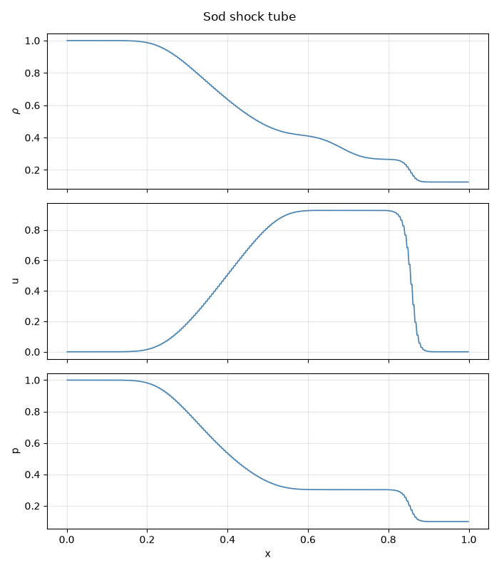
From left to right: the rarefaction fan (density and pressure falling off smoothly), the contact discontinuity (a density jump with continuous pressure and velocity – look for the density “step” where pressure and velocity stay flat), and the shock (a sharp jump in all three fields, smeared over a few cells by the scheme’s numerical diffusion).

fig, axes = plot_shock_tube_profiles(result["x"], result["rho"], result["u"], result["p"])

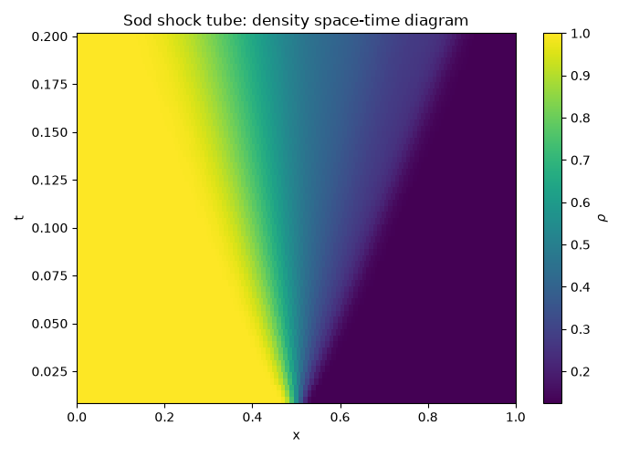
How the three waves emerge: a density space-time diagram

The single snapshot above is one horizontal slice through this picture. Re-solving sod_shock_tube() at a sequence of increasing t_final (each an independent solve from the same initial diaphragm, at a coarser resolution to keep the sweep cheap) traces out how the three waves fan out from x0 over time: the rarefaction fan spreading left as a broadening pale wedge, and the contact discontinuity and shock both running right, at their own distinct, constant speeds.

times = np.linspace(0.01, 0.2, 60)
history = [sod_shock_tube(nx=200, t_final=float(t)) for t in times]
x_coarse = history[0]["x"]
rho_history = np.array([h["rho"] for h in history])

fig, ax = plt.subplots(figsize=(7, 5))
im = ax.pcolormesh(x_coarse, times, rho_history, cmap=theme.SEQUENTIAL_CMAP, shading="auto")
fig.colorbar(im, ax=ax, label=r"$\rho$")
ax.set_xlabel("x")
ax.set_ylabel("t")
ax.set_title("Sod shock tube: density space-time diagram")
fig.tight_layout()

plt.show()