Normal shock relations across a range of Mach numbers

A normal shock is a stationary discontinuity, perpendicular to the flow, in an otherwise steady 1D inviscid compressible flow of an ideal gas: state 1 (upstream) and state 2 (downstream) must conserve mass, momentum, and energy flux across it exactly (the Rankine-Hugoniot conditions, rankine_hugoniot_jump_conditions()). Solved for an ideal gas, these give the downstream state entirely as a function of the upstream Mach number \(M_1=u_1/c_1\):

\[\frac{p_2}{p_1} = 1 + \frac{2\gamma}{\gamma+1}(M_1^2-1), \qquad \frac{\rho_2}{\rho_1} = \frac{(\gamma+1)M_1^2}{(\gamma-1)M_1^2+2}, \qquad M_2^2 = \frac{1+\tfrac{\gamma-1}{2}M_1^2}{\gamma M_1^2-\tfrac{\gamma-1}{2}},\]

as normal_shock_relations() computes. Only \(M_1\geq 1\) gives a physically admissible (entropy-increasing) shock: a normal shock always drives a supersonic upstream flow back to subsonic downstream, at the cost of a sharp jump in pressure and density. This example sweeps the upstream Mach number and plots how strongly the shock compresses the flow.

import matplotlib.pyplot as plt
import numpy as np

from physicskit.fluids.systems.compressible_flow import normal_shock_relations
from physicskit.fluids.visualizers import theme

Sweep the upstream Mach number

M1 = np.linspace(1.0, 5.0, 100)
jumps = [normal_shock_relations(m) for m in M1]
p2_p1 = np.array([j["p2_p1"] for j in jumps])
rho2_rho1 = np.array([j["rho2_rho1"] for j in jumps])
M2 = np.array([j["M2"] for j in jumps])

Plot the jump ratios

Density compresses toward a finite limit (\((\gamma+1)/(\gamma-1) = 6\) for air) even as pressure keeps climbing without bound – the shock gets thermodynamically stronger, but a perfect gas can only be squeezed so much.

fig, axes = plt.subplots(1, 2, figsize=(10, 4))
axes[0].plot(M1, p2_p1, color=theme.PRIMARY, label=r"$p_2/p_1$")
axes[0].plot(M1, rho2_rho1, color=theme.ACCENT, label=r"$\rho_2/\rho_1$")
axes[0].axhline(6.0, color=theme.MUTED, ls="--", lw=1.0, label=r"$\rho_2/\rho_1 \to 6$ as $M_1 \to \infty$")
axes[0].set_xlabel(r"$M_1$")
axes[0].legend()
axes[0].set_title("Shock jump ratios")

axes[1].plot(M1, M2, color=theme.PRIMARY)
axes[1].axhline(1.0, color=theme.MUTED, ls="--", lw=1.0)
axes[1].set_xlabel(r"$M_1$")
axes[1].set_ylabel(r"$M_2$")
axes[1].set_title("Downstream Mach number is always subsonic")
fig.tight_layout()

print(f"as M1 -> infinity, rho2/rho1 -> {rho2_rho1[-1]:.3f} (approaching the (gamma+1)/(gamma-1) = 6 limit)")

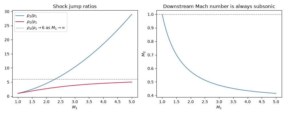
as M1 -> infinity, rho2/rho1 -> 5.000 (approaching the (gamma+1)/(gamma-1) = 6 limit)

The compression limit itself depends on the gas

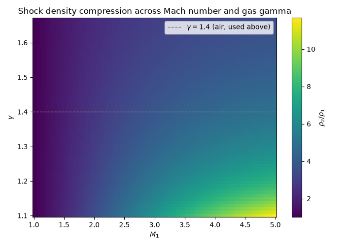
Everything above fixed \(\gamma=1.4\) (diatomic air). Sweeping \(\gamma\) too turns the single density-ratio curve into a full 2D map: the saturation value a shock approaches as \(M_1\to\infty\) is exactly \((\gamma+1)/(\gamma-1)\), so a monatomic gas (\(\gamma=5/3\), few internal degrees of freedom to soak up compression work) saturates at a much lower density ratio than a diatomic one (\(\gamma=1.4\)).

gammas = np.linspace(1.1, 5.0 / 3.0, 60)
rho_ratio_grid = np.array([[normal_shock_relations(m, gamma=g)["rho2_rho1"] for m in M1] for g in gammas])

fig, ax = plt.subplots(figsize=(7, 5))
im = ax.pcolormesh(M1, gammas, rho_ratio_grid, cmap=theme.SEQUENTIAL_CMAP, shading="auto")
fig.colorbar(im, ax=ax, label=r"$\rho_2/\rho_1$")
ax.axhline(1.4, color=theme.MUTED, ls="--", lw=1.0, label=r"$\gamma=1.4$ (air, used above)")
ax.set_xlabel(r"$M_1$")
ax.set_ylabel(r"$\gamma$")
ax.legend()
ax.set_title("Shock density compression across Mach number and gas gamma")
fig.tight_layout()

plt.show()