Richardson’s cascade: big whorls have little whorls

Richardson (1922) pictured turbulence as a hierarchy of eddies:

Big whorls have little whorls that feed on their velocity, and little whorls have lesser whorls and so on to viscosity.

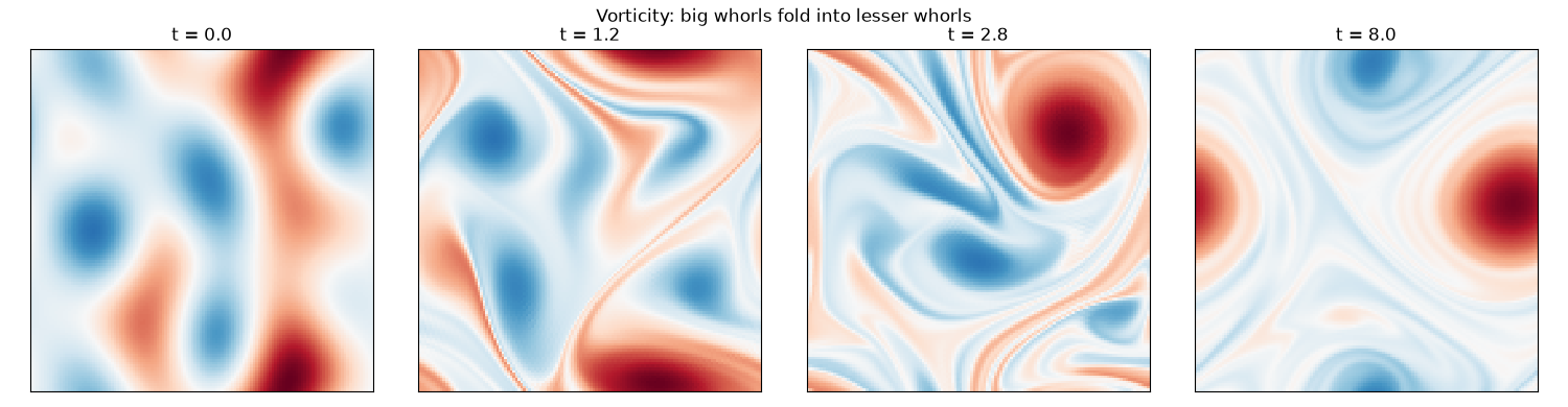
The picture is qualitative – a direction of transfer, from large scales to small, ending in viscous dissipation – with no power law attached. This example watches it happen in NavierStokes2D. The flow starts with only a few large eddies. Advection stretches and folds them into ever-thinner filaments, variance moves to ever-higher wavenumbers, and once it reaches the viscous scale it is destroyed.

In two dimensions the quantity that cascades to small scales is the enstrophy \(Z=\tfrac12\langle\omega^2\rangle\), the mean squared vorticity; the energy itself mostly stays at large scales. The qualitative picture – whorls breaking into lesser whorls until viscosity takes over – is Richardson’s.

import matplotlib.pyplot as plt
import numpy as np

from physicskit.fluids.systems.navier_stokes import NavierStokes2D
from physicskit.fluids.utils.spectral_analysis import energy_spectrum

Start with big whorls only

Random phases on the lowest few Fourier modes, \(|k|\le 3\): a handful of domain-sized eddies and nothing smaller.

n, length = 128, 2 * np.pi
solver = NavierStokes2D(n=n, length=length, nu=1.5e-3)

rng = np.random.default_rng(1922)
omega = np.zeros_like(solver.X)
for kx in range(-3, 4):
    for ky in range(0, 4):
        if kx**2 + ky**2 == 0 or kx**2 + ky**2 > 9:
            continue
        omega += rng.normal() * np.cos(kx * solver.X + ky * solver.Y + rng.uniform(0, 2 * np.pi))
omega *= 5.0 / omega.std()

Evolve and record

Snapshots of the vorticity, its enstrophy spectrum \(Z(k)=k^2E(k)\), and the enstrophy-weighted mean wavenumber \(\bar k = \sum kZ(k)/\sum Z(k)\) – the inverse size of a typical whorl.

dt, steps_per_chunk, n_chunks = 0.004, 50, 40
snap_every = {0: None, 6: None, 14: None, 40: None}
times, k_mean, Z_total = [], [], []
spectra = {}
for chunk in range(n_chunks + 1):
    t = chunk * steps_per_chunk * dt
    res = solver.simulate(omega, dt=dt, steps=0)
    k, E = energy_spectrum(res["u"], res["v"], length)
    Zk = k**2 * E
    times.append(t)
    k_mean.append(np.sum(k * Zk) / np.sum(Zk))
    Z_total.append(0.5 * np.mean(omega**2))
    if chunk in snap_every:
        snap_every[chunk] = omega.copy()
        spectra[t] = (k, Zk)
    if chunk < n_chunks:
        omega = solver.simulate(omega, dt=dt, steps=steps_per_chunk)["omega"]

fig1, axes = plt.subplots(1, 4, figsize=(15, 3.9))
vmax = np.abs(snap_every[0]).max()
for ax, (chunk, w) in zip(axes, snap_every.items()):
    ax.pcolormesh(solver.X, solver.Y, w, cmap="RdBu_r", vmin=-vmax, vmax=vmax, shading="auto")
    ax.set_title(f"t = {chunk * steps_per_chunk * dt:.1f}")
    ax.set_aspect("equal")
    ax.set_xticks([])
    ax.set_yticks([])
fig1.suptitle("Vorticity: big whorls fold into lesser whorls")
fig1.tight_layout()

Variance marches to small scales, then viscosity takes it

The enstrophy spectrum spreads from \(k\le3\) to the dissipation range and the typical whorl shrinks (\(\bar k\) rises). Total enstrophy falls fastest while \(\bar k\) is high: viscosity acts at the bottom of the cascade, on the small whorls, not on the large eddies the flow started with. Once the small scales are drained, the few surviving large vortices decay slowly.

i_peak = int(np.argmax(k_mean))
print(f"mean enstrophy wavenumber: {k_mean[0]:.2f} at t=0 -> peak {k_mean[i_peak]:.2f} at t={times[i_peak]:.2f}")
print(f"enstrophy: {Z_total[0]:.3f} at t=0, {Z_total[i_peak]:.3f} at the peak, {Z_total[-1]:.3f} at t={times[-1]:.1f}")

fig2, (ax2, ax3) = plt.subplots(1, 2, figsize=(11, 4))
for (t, (k, Zk)), color in zip(spectra.items(), plt.cm.viridis(np.linspace(0, 0.9, len(spectra)))):
    ax2.loglog(k[1:], Zk[1:], color=color, label=f"t = {t:.1f}")
ax2.set_ylim(1e-8, None)
ax2.set_xlabel("wavenumber k")
ax2.set_ylabel(r"enstrophy spectrum $k^2E(k)$")
ax2.set_title("Spreading to small scales")
ax2.legend(fontsize=8)

ax3.plot(times, k_mean, color="steelblue")
ax3.set_xlabel("t")
ax3.set_ylabel(r"$\bar k$ (inverse whorl size)", color="steelblue")
ax3b = ax3.twinx()
ax3b.plot(times, Z_total, color="firebrick")
ax3b.set_ylabel("total enstrophy", color="firebrick")
ax3.set_title("Whorls shrink, then viscosity wins")
fig2.tight_layout()

plt.show()

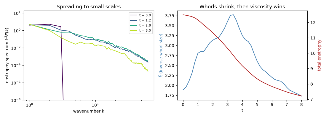
mean enstrophy wavenumber: 1.89 at t=0 -> peak 3.77 at t=3.40
enstrophy: 12.500 at t=0, 9.850 at the peak, 7.218 at t=8.0

Check

Whorls break into smaller whorls (the mean enstrophy wavenumber doubles) while total enstrophy can only decrease in 2D viscous flow.

assert k_mean[i_peak] > 1.8 * k_mean[0]
assert np.all(np.diff(Z_total) <= 1e-9)