The Kolmogorov -5/3 cascade in forced 2D turbulence

Kolmogorov’s 1941 theory concerns turbulence in a statistical steady state: energy is injected at some scale at a rate \(\varepsilon\), passed through an “inertial range” of scales by the nonlinear terms alone, and removed elsewhere. If the statistics there depend only on \(\varepsilon\) and the wavenumber \(k\), dimensional analysis fixes the energy spectrum,

\[E(k) = C\,\varepsilon^{2/3} k^{-5/3}.\]

A cascade needs a steady flux, so this example forces the flow rather than letting it decay. ForcedTurbulence2D injects energy at the fixed rate \(\varepsilon\) on a shell of wavenumbers around \(k_f = 20\) on a \(128^2\) periodic grid. 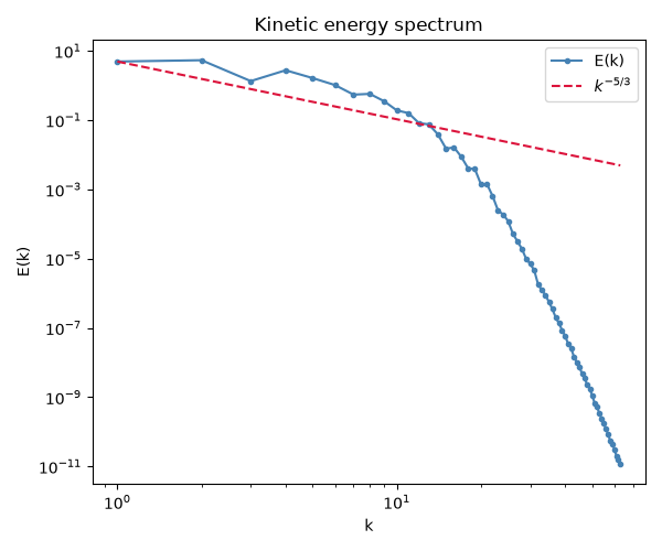In two dimensions the energy flows to larger scales (Kraichnan’s inverse cascade), where a weak linear drag removes it, so the Kolmogorov range lies at \(k < k_f\); the enstrophy cascades the other way, to \(E \propto k^{-3}\) above \(k_f\). The time-averaged spectrum is compared with the \(-5/3\) law.

import matplotlib.pyplot as plt
import numpy as np

from physicskit.fluids.systems.turbulence import ForcedTurbulence2D, kolmogorov_kraichnan_spectrum

flow = ForcedTurbulence2D(n=128, kf=20.0, epsilon=1.0, drag=0.1, seed=0)
out = flow.run(t_max=20.0, dt=0.004, t_average=10.0)
k, E = out["k"], out["E"]

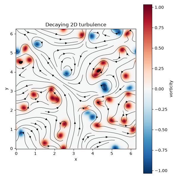
Vorticity and energy budget

fig, axes = plt.subplots(1, 3, figsize=(14, 4.3))
x = np.linspace(0, 2 * np.pi, flow.n, endpoint=False)
vmax = np.percentile(np.abs(out["omega"]), 99)
axes[0].pcolormesh(x, x, out["omega"], cmap="RdBu_r", vmin=-vmax, vmax=vmax, shading="auto")
axes[0].set_aspect("equal")
axes[0].set_title(f"Vorticity at t = {out['t'][-1]:.0f}")
axes[0].set_xticks([])
axes[0].set_yticks([])

axes[1].plot(out["t"], out["energy"], color="navy")
axes[1].plot(out["t"][:30], flow.epsilon * out["t"][:30], "k--", lw=1, label=r"$\varepsilon t$")
axes[1].axvspan(out["t"][-1] - 10.0, out["t"][-1], color="gray", alpha=0.15, label="averaging window")
axes[1].set_xlabel("t")
axes[1].set_ylabel("kinetic energy")
axes[1].set_title("Energy grows at the injection rate, then saturates")
axes[1].legend()

<matplotlib.legend.Legend object at 0x130bea3c0>

The time-averaged spectrum

inertial = (k >= 3) & (k <= 12)
slope, intercept = np.polyfit(np.log(k[inertial]), np.log(E[inertial]), 1)
C = np.median(E[inertial] * k[inertial] ** (5 / 3)) / flow.epsilon ** (2 / 3)
axes[2].loglog(k[1:], E[1:], color="navy", label="measured")
kk = k[inertial]
axes[2].loglog(kk, kolmogorov_kraichnan_spectrum(kk, flow.epsilon, C) * 1.6, "k--", label=r"$k^{-5/3}$")
ks = np.arange(25, 40)
axes[2].loglog(ks, E[25] * (ks / 25.0) ** -3 * 0.6, "k:", label=r"$k^{-3}$")
axes[2].axvline(flow.kf, color="crimson", lw=0.8, label=r"forcing $k_f$")
axes[2].set_ylim(E[1:60].min() / 3, E[1:].max() * 3)
axes[2].set_xlabel("k")
axes[2].set_ylabel("E(k)")
axes[2].set_title(f"Fitted slope {slope:.2f} for 3 <= k <= 12")
axes[2].legend(fontsize=8)
plt.tight_layout()
plt.show()
print(f"inertial-range slope = {slope:.3f} (K41: {-5 / 3:.3f}), C = {C:.1f}")

inertial-range slope = -1.686 (K41: -1.667), C = 3.7

Check

The inverse-cascade range follows the Kolmogorov exponent.

assert abs(slope + 5 / 3) < 0.15