Stokes drag and the terminal velocity of a settling sphere

In the creeping-flow limit \(Re = 2R|v|/\nu \ll 1\), the nonlinear advection term in the Navier-Stokes equations is negligible next to viscous diffusion, leaving the linear Stokes equations \(\mu\nabla^2\mathbf{u}=\nabla p\) – George Stokes’ 1851 exact solution for uniform flow past a sphere of radius \(R\), giving a drag force

\[F_D = 6\pi\mu R v.\]

A sphere of density \(\rho_s\) settling under gravity through a fluid of density \(\rho_f\) and viscosity \(\mu\) reaches a terminal velocity \(v\) where this drag exactly balances its net (gravity minus buoyancy) weight,

\[6\pi\mu R v = \tfrac{4}{3}\pi R^3 (\rho_s - \rho_f)\,g.\]

This example solves that balance for the terminal velocity across a range of sphere radii and checks, via reynolds_number(), that Stokes’ law remains a good approximation only while the resulting Reynolds number stays small – exactly the regime the law assumes.

import matplotlib.pyplot as plt
import numpy as np

from physicskit.fluids.systems.viscous_flow import stokes_drag
from physicskit.fluids.utils.dimensionless import reynolds_number
from physicskit.fluids.visualizers import theme

Solve for the terminal velocity at each radius

At terminal velocity, Stokes drag balances net weight: \(6\pi\mu R v = \tfrac{4}{3}\pi R^3 (\rho_s - \rho_f) g\).

mu, rho_fluid, rho_sphere, g = 1.0e-3, 1000.0, 2500.0, 9.81  # water, glass bead
radii = np.geomspace(1e-5, 1e-3, 40)
net_weight = (4.0 / 3.0) * np.pi * radii**3 * (rho_sphere - rho_fluid) * g
v_terminal = net_weight / np.array([stokes_drag(mu, R, 1.0) for R in radii])

nu = mu / rho_fluid
Re = np.array([reynolds_number(velocity=v, length=2 * R, nu=nu) for v, R in zip(v_terminal, radii)])

Plot terminal velocity and its Reynolds number

The Reynolds number rises sharply with radius; Stokes’ law is only self-consistent while it stays well below 1.

fig, axes = plt.subplots(1, 2, figsize=(10, 4))
axes[0].loglog(radii, v_terminal, color=theme.PRIMARY, marker="o", markersize=3)
axes[0].set_xlabel("sphere radius (m)")
axes[0].set_ylabel("terminal velocity (m/s)")
axes[0].set_title("Stokes terminal velocity")

axes[1].loglog(radii, Re, color=theme.ACCENT, marker="o", markersize=3)
axes[1].axhline(1.0, color=theme.MUTED, ls="--", lw=1.0, label="Re = 1 (Stokes' law breaks down)")
axes[1].set_xlabel("sphere radius (m)")
axes[1].set_ylabel("Reynolds number")
axes[1].legend()
axes[1].set_title("Validity of Stokes' law")
fig.tight_layout()

valid = Re < 1.0
print(f"Stokes' law is self-consistent (Re < 1) for radii up to {radii[valid][-1] * 1e6:.1f} microns")

plt.show()

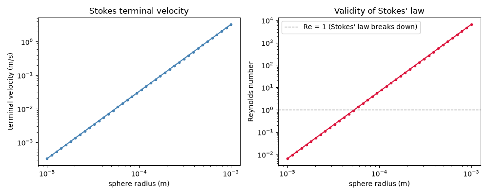
Stokes' law is self-consistent (Re < 1) for radii up to 52.2 microns